
Intro to ggplot2
Grayson White
Math 141
Week 2 | Fall 2025
Load Necessary Packages
ggplot2 is part of this collection of data science packages.
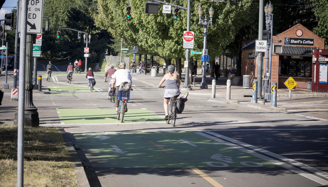
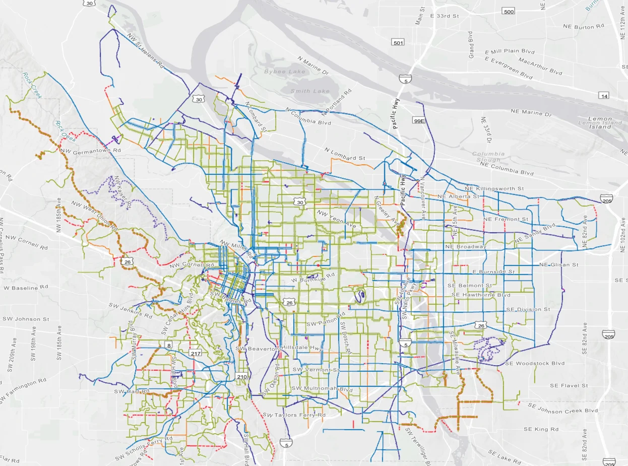
Data Setting: Portland Bikeshare Data
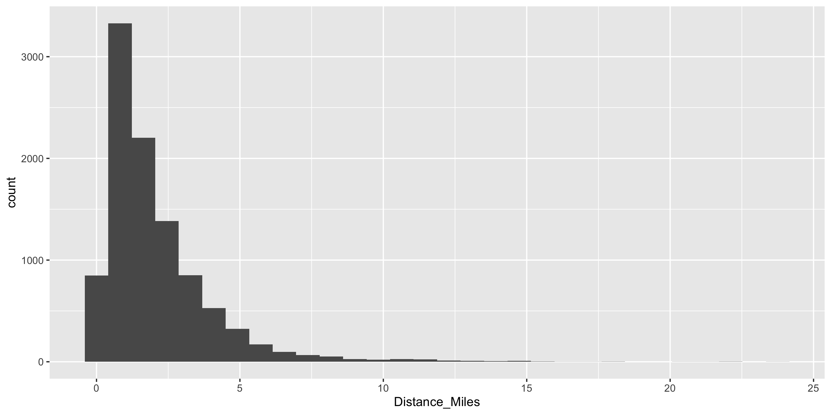
Histograms
Binned counts of data.
Great for assessing shape.
Question: are histograms used for quantitative or categorical variables?
Answer: Quantitative.

Data Shapes
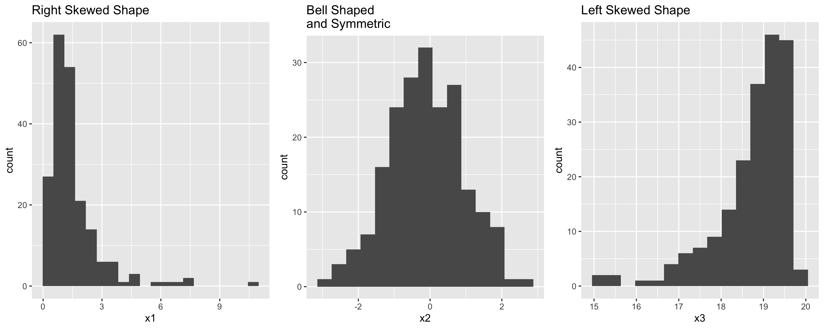
Histograms
Histograms
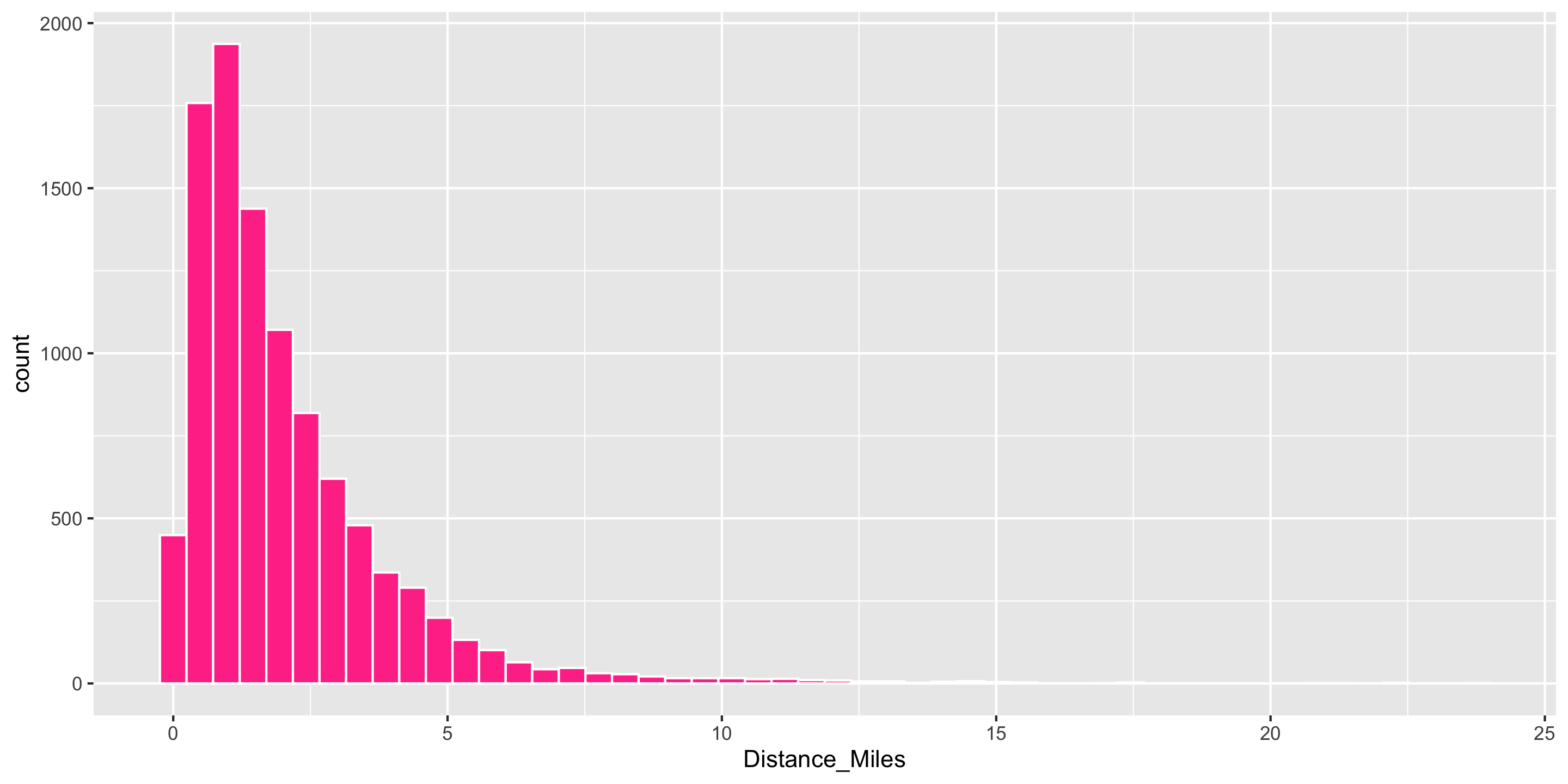
- mapping to a variable goes in
aes() - setting to a specific value goes in the
geom_---()
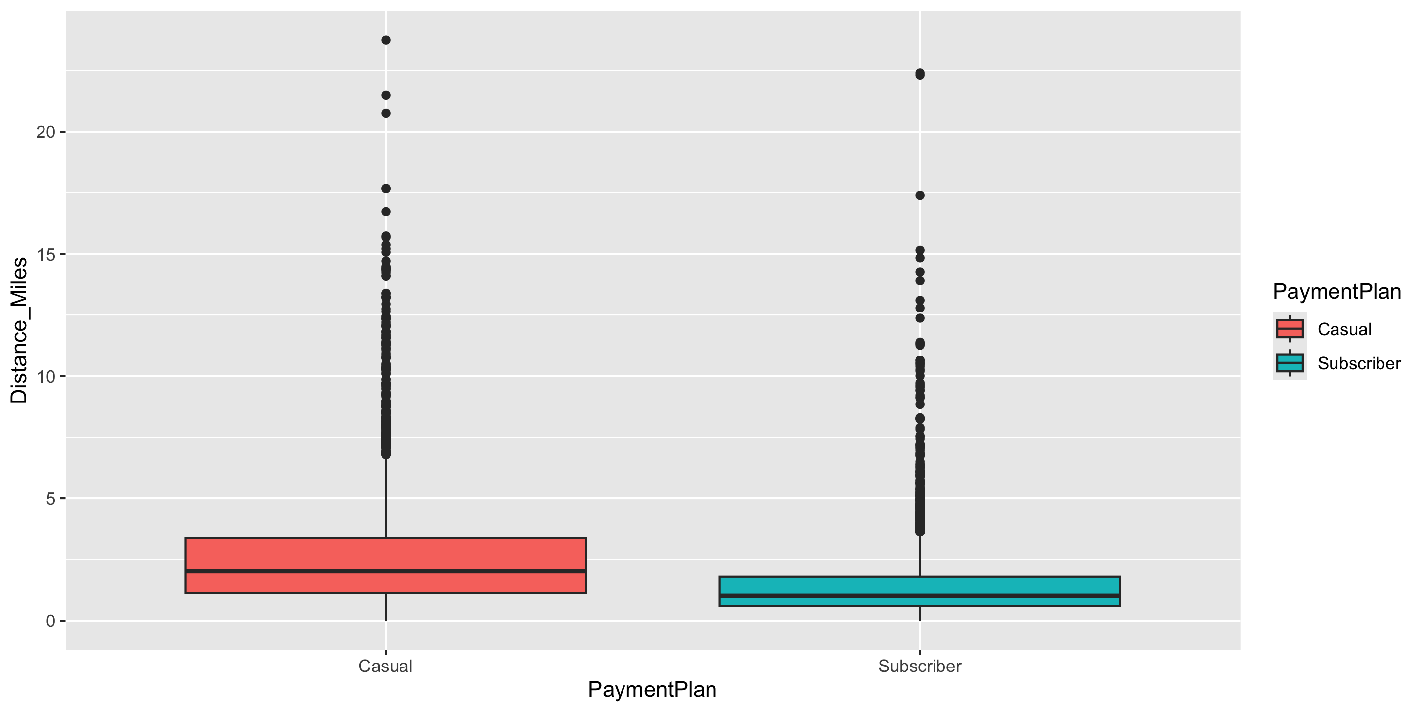
Boxplots
- Five number summary:
- Minimum
- First quartile (Q1)
- Median
- Third quartile (Q3)
- Maximum
- Interquartile range (IQR) \(=\) Q3 \(-\) Q1
- Outliers: unusual points
- Boxplot defines unusual as being beyond \(1.5*IQR\) from \(Q1\) or \(Q3\).
- Whiskers: reach out to the furthest point that is NOT an outlier
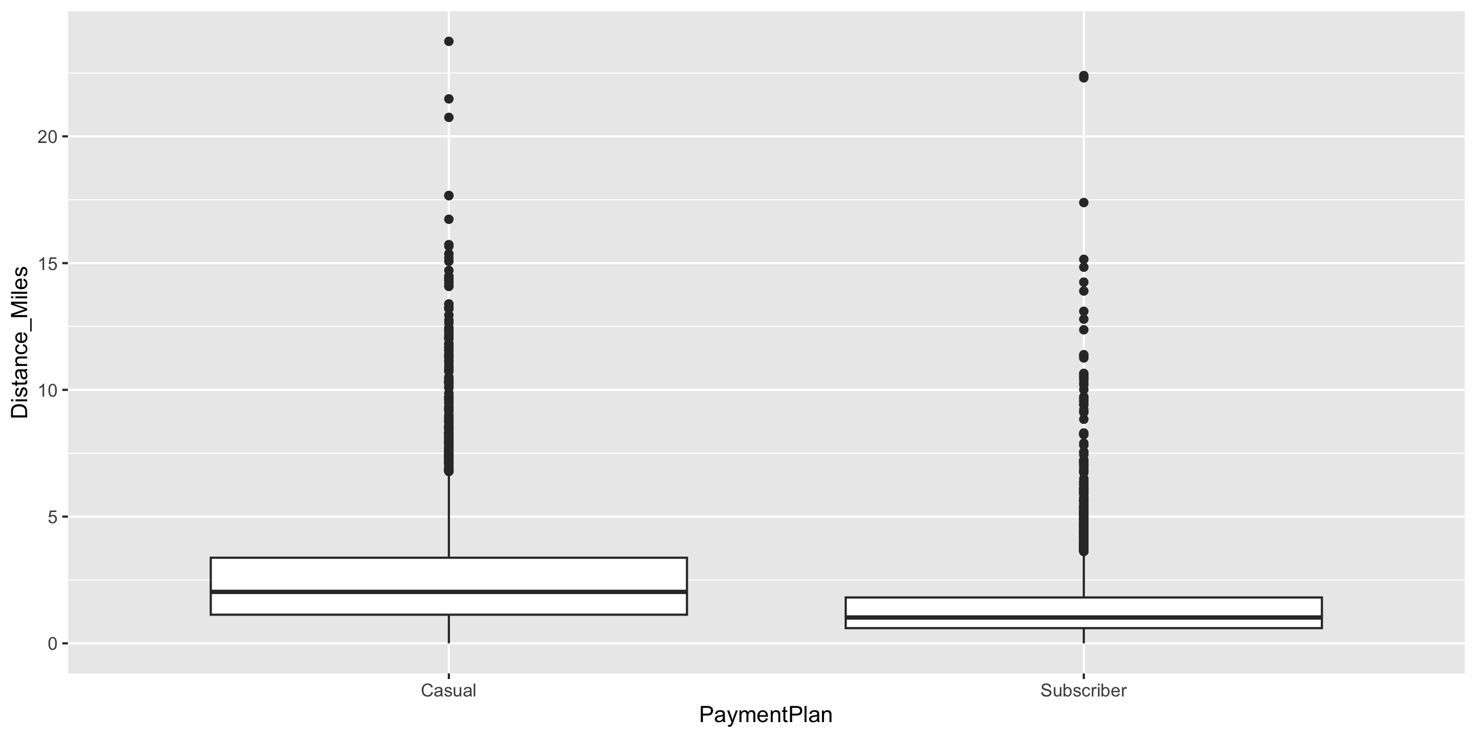
Boxplots

Boxplots
- Is this
fillanaesthetic mapping?
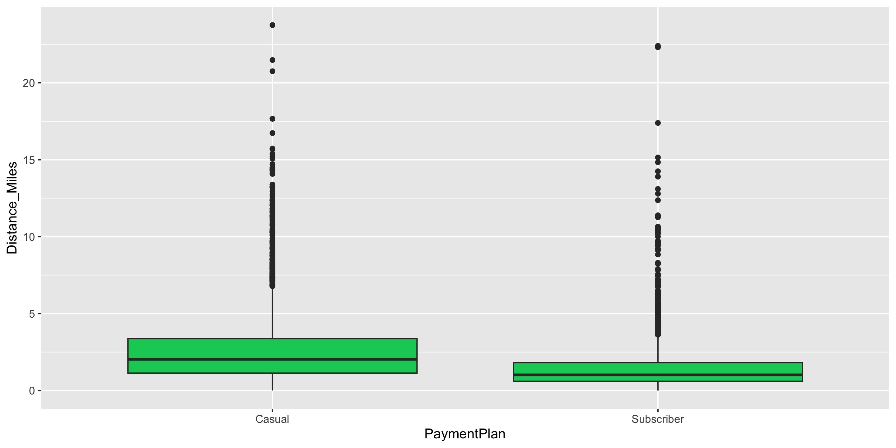
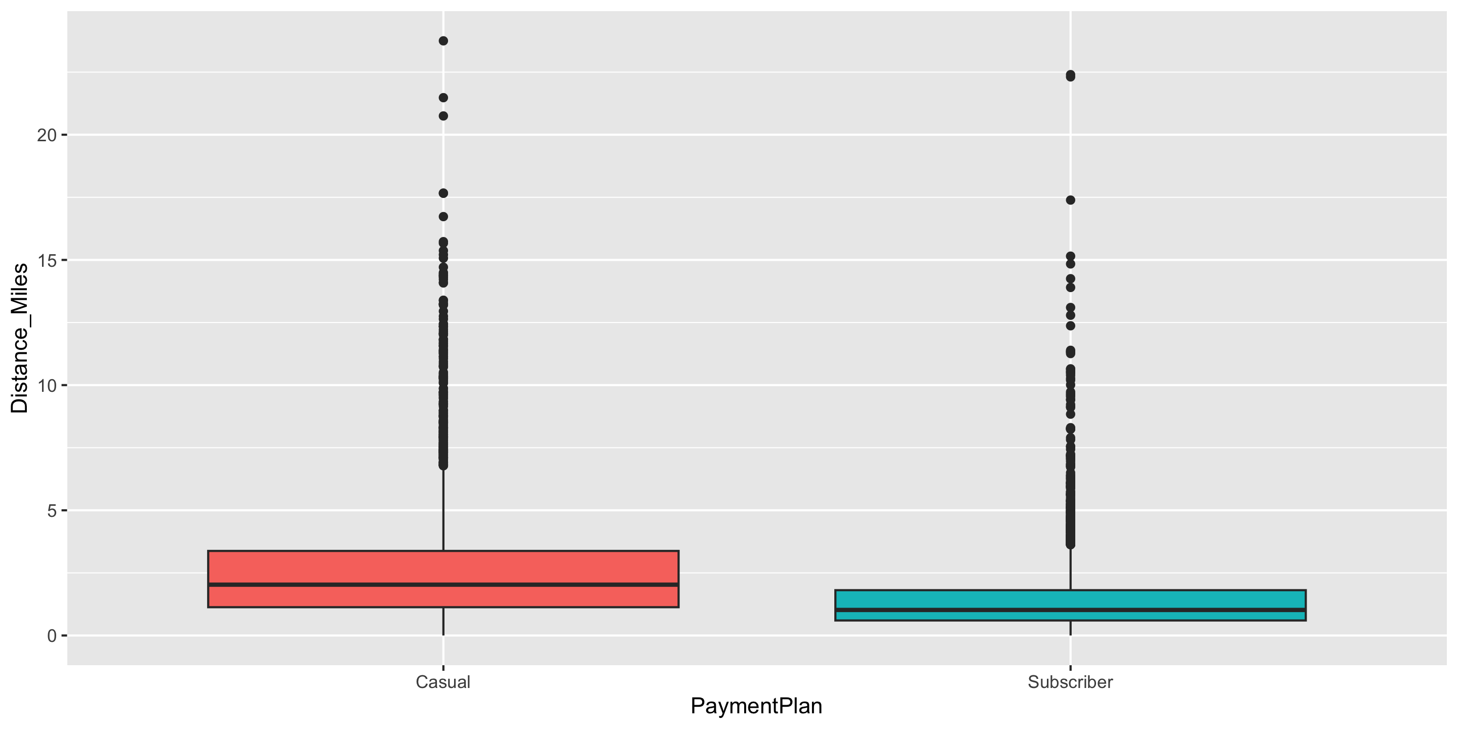
Boxplots
Is this
fillanaesthetic mapping?What variable is mapped to
fill?
Boxplots
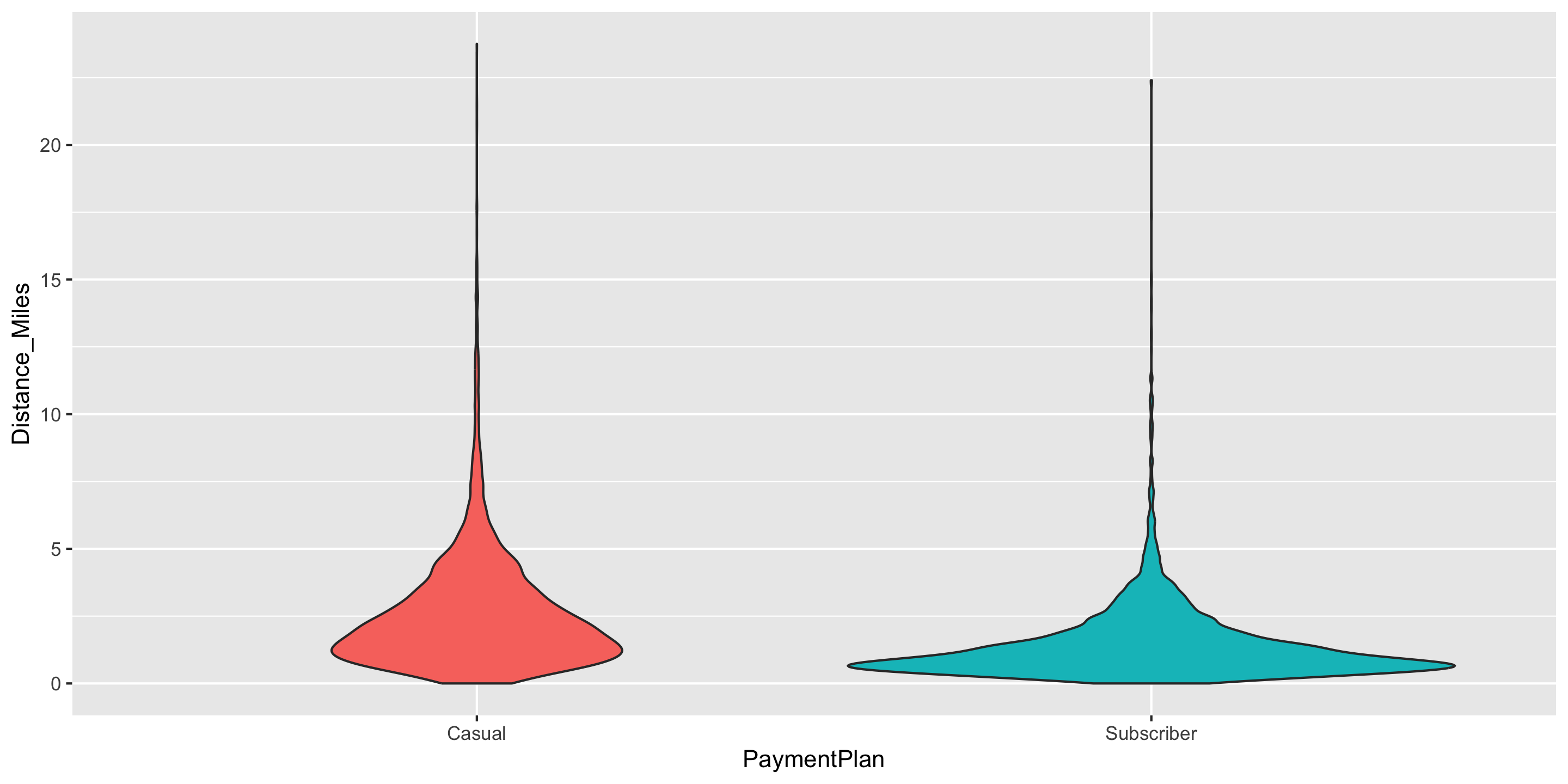
Violin Plots

Boxplot Versus Violin Plots

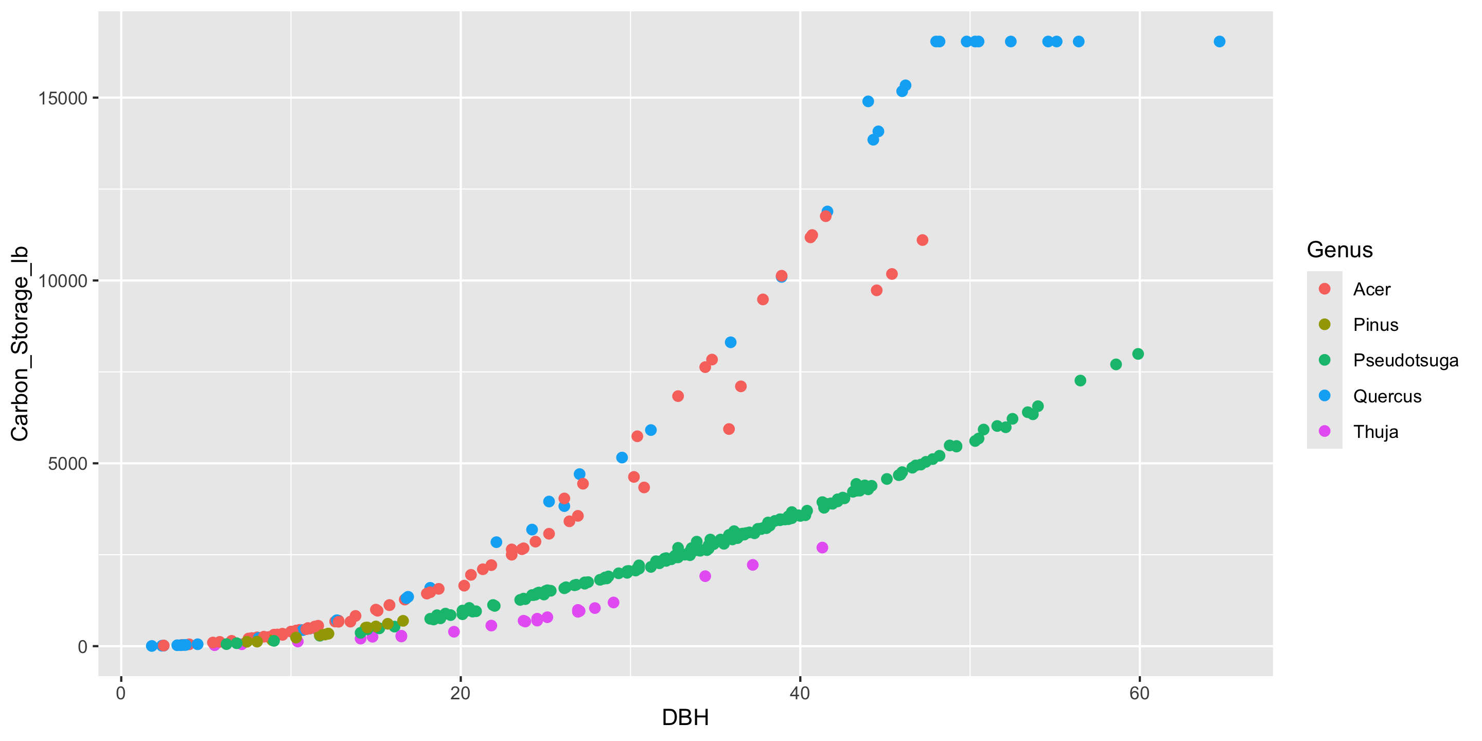
Scatterplots
- Explore relationships between numerical variables.
- We will be especially interested in linear relationships.
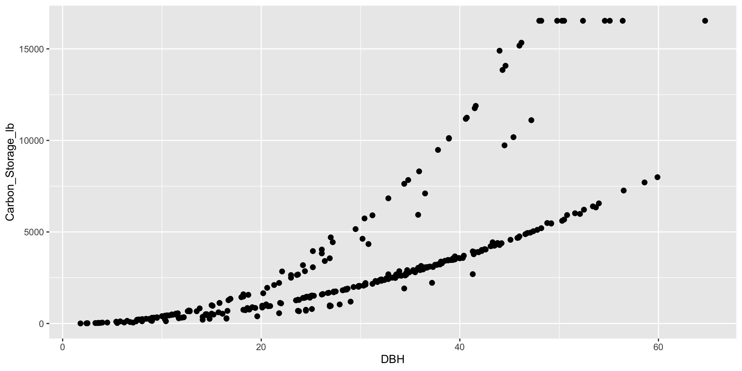
Scatterplots
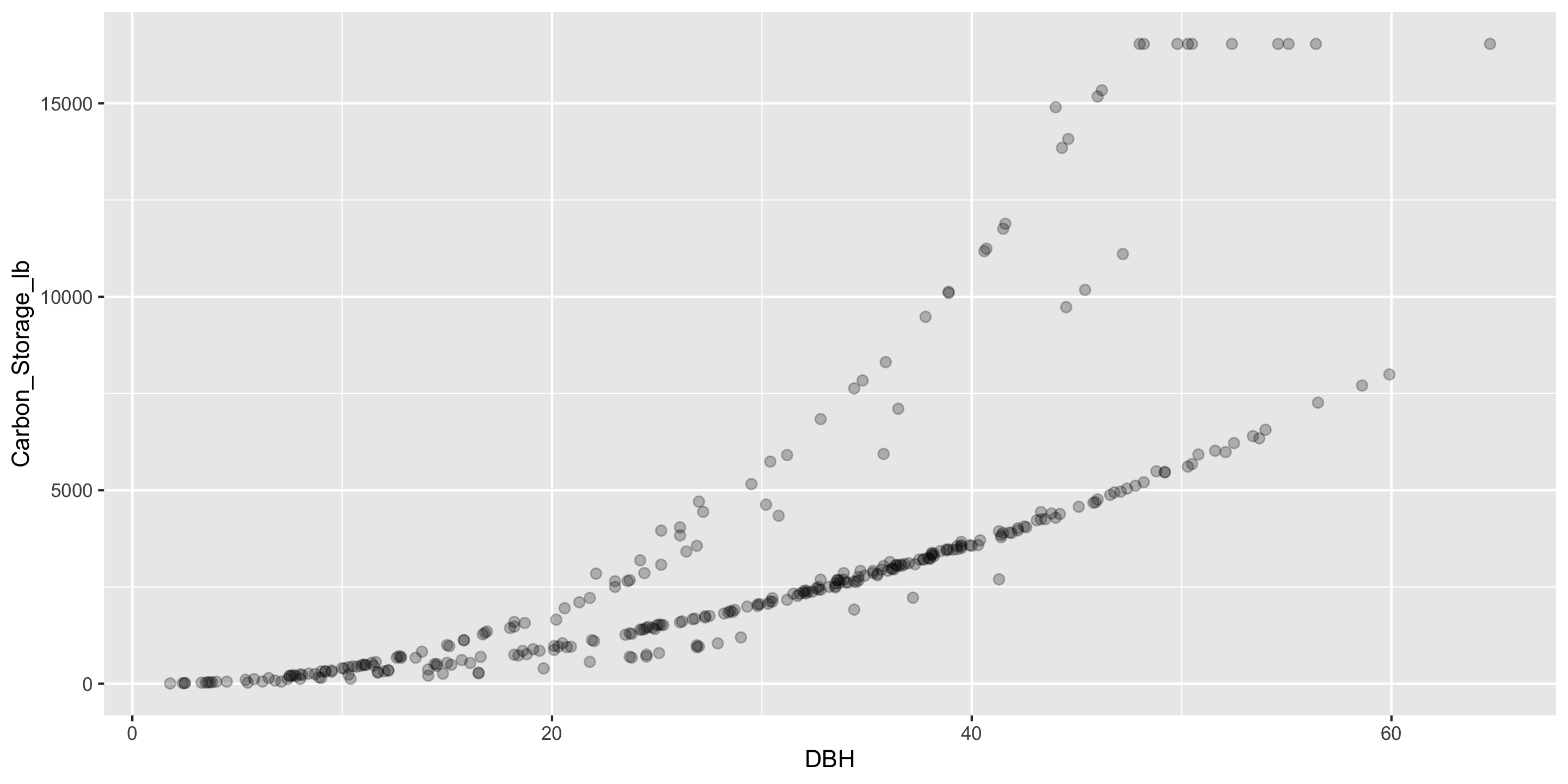
- Fix over-plotting
- What’s going on in this graph?
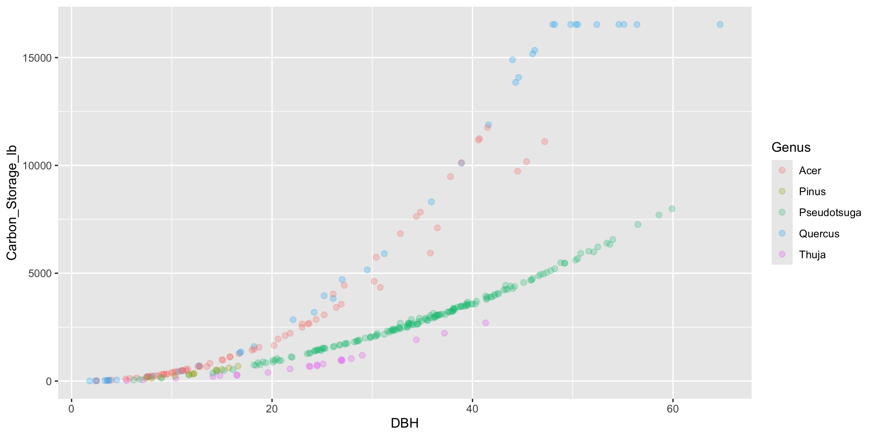
Scatterplots
Linegraphs
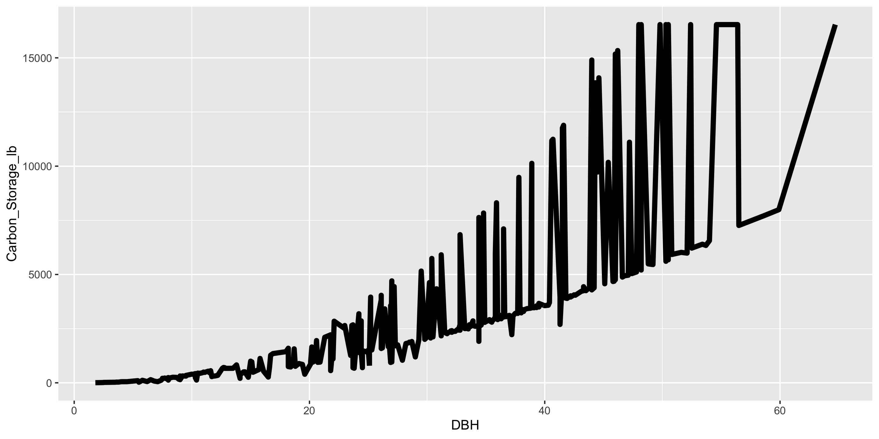
Linegraphs
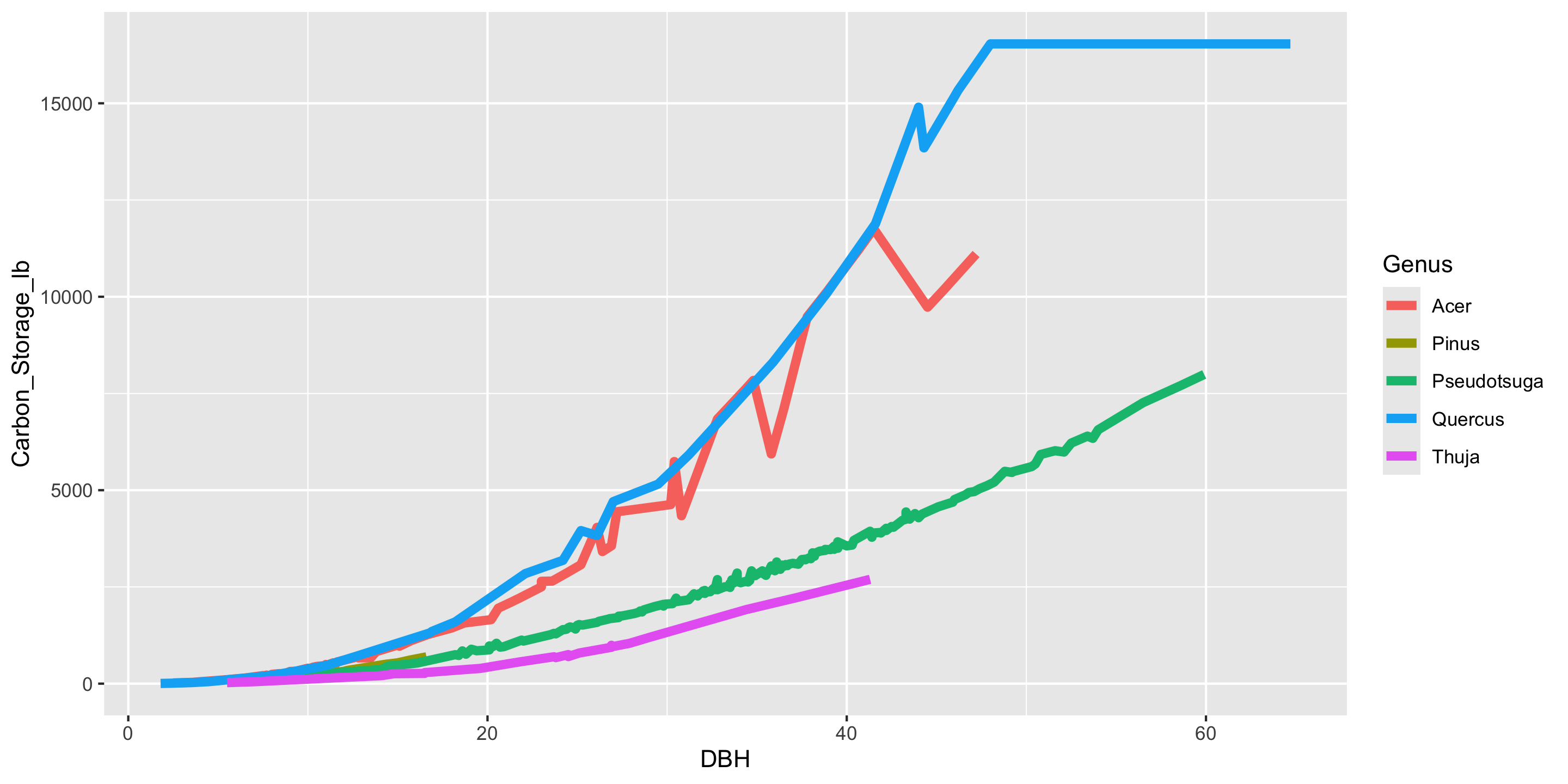
Linegraphs vs scatterplots

- Which do you prefer?
- Does it depend on context?
- Which might be better if we put time on the x-axis?