
Data Wrangling with dplyr
Grayson White
Math 141
Week 3 | Fall 2025
Goals For Today
- Learn to wrangle data with
dplyr!
Load Necessary Packages

dplyr is part of this collection of data science packages.
Data for today
dogs <- read_csv("https://data.cambridgema.gov/api/views/sckh-3xyx/rows.csv")

# Useful wrangling that we will come back to
dogs_top5 <- dogs %>%
  mutate(Breed = case_when(
                       Dog_Breed == "Mixed Breed" ~ "Mixed",
                       Dog_Breed != "Mixed Breed" ~ "Single")) %>%
  filter(Dog_Name %in% c("Luna", "Charlie", "Lucy", "Cooper", "Rosie" ))
Data for today
Rows: 1,581
Columns: 6
$ Dog_Name         <chr> "Thor", "Lucy", "Ruby", "Georgie", "Candy", "kylo-roo…
$ Dog_Breed        <chr> "Boxer", "Poodle", "Collie", "Lhasa Apso", "Beagle", …
$ Location_masked  <lgl> NA, NA, NA, NA, NA, NA, NA, NA, NA, NA, NA, NA, NA, N…
$ Latitude_masked  <dbl> 42.3622, 42.3696, 42.3860, 42.3742, 42.3918, 42.3862,…
$ Longitude_masked <dbl> -71.0846, -71.1109, -71.1237, -71.1418, -71.1290, -71…
$ Neighborhood <chr> "East Cambridge", "Mid-Cambridge", "Neighborhood Nine…Rows: 57
Columns: 7
$ Dog_Name <chr> "Lucy", "Luna", "Charlie", "Cooper", "Charlie", "Luna…
$ Dog_Breed <chr> "Poodle", "LABRADOODLE", "Border Terrier Mix", "Germa…
$ Location_masked <lgl> NA, NA, NA, NA, NA, NA, NA, NA, NA, NA, NA, NA, NA, N…
$ Latitude_masked <dbl> 42.3696, 42.3860, 42.3596, 42.3573, 42.3895, 42.3913,…
$ Longitude_masked <dbl> -71.1109, -71.1362, -71.1143, -71.1015, -71.1311, -71…
$ Neighborhood <chr> "Mid-Cambridge", "Neighborhood Nine", "Cambridgeport"…
$ Breed <chr> "Single", "Single", "Single", "Single", "Single", "Mi…Data Wrangling: Transformations done on the data
Why wrangle the data?
To summarize the data.
→ To compute the mean and standard deviation of miles ridden by bikeshare users.
To drop missing values. (Need to be careful here!)
→ On our Lab 2, we are seeing that ggplot2 will often drop observations before creating a graph.
To filter to a particular subset of the data.
→ To subset the pdxTrees data to just a few species types.
To collapse the categories of a categorical variable.
→ To go from 86 dog breeds to just mixed or single breed.
Data Wrangling: Transformations done on the data
Why wrangle the data?
To arrange the data to make it easier to display.
→ To sort from most common dog name to least common.
To fix how R stores a variable.
→ Converting quantitative variables to/from categorical variables
dplyr for Data Wrangling
- Six common wrangling verbs:
summarize()count()
mutate()
select()filter()arrange()
- One action:
group_by()
Return to mutate()
Add new variables
# A tibble: 10 × 4
# Groups:   Dog_Name [5]
   Dog_Name Breed      n  prop
   <chr>    <chr>  <int> <dbl>
 1 Charlie  Mixed      4 0.286
 2 Charlie  Single    10 0.714
 3 Cooper   Mixed      1 0.125
 4 Cooper   Single     7 0.875
 5 Lucy     Mixed      2 0.182
 6 Lucy     Single     9 0.818
 7 Luna     Mixed      7 0.5
 8 Luna     Single     7 0.5
 9 Rosie    Mixed      1 0.1
10 Rosie Single 9 0.9 select(): Extract variables
# A tibble: 1,581 × 2
   Dog_Name Dog_Breed
   <chr>    <chr>
 1 Thor     Boxer
 2 Lucy     Poodle
 3 Ruby     Collie
 4 Georgie  Lhasa Apso
 5 Candy    Beagle
 6 kylo-roo chihuahua yorkie mix
 7 Sandy    Cocker Spaniel
 8 Willy    Labraddoodle
 9 yoshi    plotthound pit mix
10 Colby    Cocker Spaniel
# ℹ 1,571 more rows
Motivation for filter()
filter(): Extract cases
arrange(): Sort the cases
New Data Setting: Bureau of Labor Statistics (BLS) Consumer Expenditure Survey
BLS Mission: “Measures labor market activity, working conditions, price changes, and productivity in the U.S. economy to support public and private decision making.”
Data: Last quarter of the 2016 BLS Consumer Expenditure Survey.
Rows: 6,301
Columns: 51
$ NEWID    <chr> "03324174", "03324204", "03324214", "03324244", "03324274", "…
$ PRINEARN <chr> "01", "01", "01", "01", "02", "01", "01", "01", "02", "01", "…
$ FINLWT21 <dbl> 25984.767, 6581.018, 20208.499, 18078.372, 20111.619, 19907.3…
$ FINCBTAX <dbl> 116920, 200, 117000, 0, 2000, 942, 0, 91000, 95000, 40037, 10…
$ BLS_URBN <dbl> 1, 1, 1, 1, 1, 1, 1, 1, 2, 1, 1, 1, 1, 1, 1, 1, 1, 1, 1, 1, 1…
$ POPSIZE  <dbl> 2, 3, 4, 2, 2, 2, 1, 2, 5, 2, 3, 2, 2, 3, 4, 3, 3, 1, 4, 1, 1…
$ EDUC_REF <chr> "16", "15", "16", "15", "14", "11", "10", "13", "12", "12", "…
$ EDUCA2   <dbl> 15, 15, 13, NA, NA, NA, NA, 15, 15, 14, 12, 12, NA, NA, NA, 1…
$ AGE_REF  <dbl> 63, 50, 47, 37, 51, 63, 77, 37, 51, 64, 26, 59, 81, 51, 67, 4…
$ AGE2     <dbl> 50, 47, 46, NA, NA, NA, NA, 36, 53, 67, 44, 62, NA, NA, NA, 4…
$ SEX_REF  <dbl> 1, 1, 2, 1, 2, 1, 2, 1, 1, 2, 2, 2, 2, 2, 2, 2, 2, 2, 1, 2, 1…
$ SEX2     <dbl> 2, 2, 1, NA, NA, NA, NA, 2, 2, 1, 1, 1, NA, NA, NA, 1, NA, 1,…
$ REF_RACE <dbl> 1, 4, 2, 1, 1, 1, 1, 1, 1, 1, 1, 1, 1, 1, 1, 2, 1, 1, 1, 1, 1…
$ RACE2    <dbl> 1, 4, 1, NA, NA, NA, NA, 1, 1, 1, 1, 1, NA, NA, NA, 2, NA, 1,…
$ HISP_REF <dbl> 2, 2, 2, 2, 2, 1, 1, 2, 2, 2, 2, 2, 2, 2, 2, 2, 2, 2, 2, 1, 1…
$ HISP2    <dbl> 2, 2, 1, NA, NA, NA, NA, 2, 2, 2, 2, 2, NA, NA, NA, 2, NA, 2,…
$ FAM_TYPE <dbl> 3, 4, 1, 8, 9, 9, 8, 3, 1, 1, 3, 1, 8, 9, 8, 5, 9, 4, 8, 3, 2…
$ MARITAL1 <dbl> 1, 1, 1, 5, 3, 3, 2, 1, 1, 1, 1, 1, 2, 3, 5, 1, 3, 1, 3, 1, 1…
$ REGION   <dbl> 4, 4, 3, 4, 4, 3, 4, 1, 3, 2, 1, 4, 1, 3, 3, 3, 2, 1, 2, 4, 3…
$ SMSASTAT <dbl> 1, 1, 1, 1, 1, 1, 1, 1, 2, 1, 1, 1, 1, 1, 1, 1, 1, 1, 1, 1, 1…
$ HIGH_EDU <chr> "16", "15", "16", "15", "14", "11", "10", "15", "15", "14", "…
$ EHOUSNGC <dbl> 0, 0, 0, 0, 0, 0, 0, 0, 0, 0, 0, 0, 0, 0, 0, 0, 0, 0, 0, 0, 0…
$ TOTEXPCQ <dbl> 0, 0, 0, 0, 0, 0, 0, 0, 0, 0, 0, 0, 0, 0, 0, 0, 0, 0, 0, 0, 0…
$ FOODCQ   <dbl> 0, 0, 0, 0, 0, 0, 0, 0, 0, 0, 0, 0, 0, 0, 0, 0, 0, 0, 0, 0, 0…
$ TRANSCQ  <dbl> 0, 0, 0, 0, 0, 0, 0, 0, 0, 0, 0, 0, 0, 0, 0, 0, 0, 0, 0, 0, 0…
$ HEALTHCQ <dbl> 0, 0, 0, 0, 0, 0, 0, 0, 0, 0, 0, 0, 0, 0, 0, 0, 0, 0, 0, 0, 0…
$ ENTERTCQ <dbl> 0, 0, 0, 0, 0, 0, 0, 0, 0, 0, 0, 0, 0, 0, 0, 0, 0, 0, 0, 0, 0…
$ EDUCACQ  <dbl> 0, 0, 0, 0, 0, 0, 0, 0, 0, 0, 0, 0, 0, 0, 0, 0, 0, 0, 0, 0, 0…
$ TOBACCCQ <dbl> 0, 0, 0, 0, 0, 0, 0, 0, 0, 0, 0, 0, 0, 0, 0, 0, 0, 0, 0, 0, 0…
$ STUDFINX <dbl> NA, NA, NA, NA, NA, NA, NA, NA, NA, NA, NA, NA, NA, NA, NA, N…
$ IRAX     <dbl> 1000000, 10000, 0, NA, NA, 0, 0, 15000, NA, 477000, NA, NA, N…
$ CUTENURE <dbl> 1, 1, 1, 1, 1, 2, 4, 1, 1, 2, 1, 2, 2, 2, 2, 4, 1, 1, 1, 4, 4…
$ FAM_SIZE <dbl> 4, 6, 2, 1, 2, 2, 1, 5, 2, 2, 4, 2, 1, 2, 1, 4, 2, 4, 1, 3, 3…
$ VEHQ     <dbl> 3, 5, 0, 4, 2, 0, 0, 2, 4, 2, 3, 2, 1, 3, 1, 2, 4, 4, 0, 2, 3…
$ ROOMSQ   <dbl> 8, 5, 6, 4, 4, 4, 7, 5, 4, 9, 6, 10, 4, 7, 5, 6, 6, 8, 18, 4,…
$ INC_HRS1 <dbl> 40, 40, 40, 44, 40, NA, NA, 40, 40, NA, 40, NA, NA, NA, NA, 4…
$ INC_HRS2 <dbl> 30, 40, 52, NA, NA, NA, NA, 40, 40, NA, 65, NA, NA, NA, NA, 6…
$ EARNCOMP <dbl> 3, 2, 2, 1, 4, 7, 8, 2, 2, 8, 2, 8, 8, 7, 8, 2, 7, 3, 1, 2, 1…
$ NO_EARNR <dbl> 4, 2, 2, 1, 2, 1, 0, 2, 2, 0, 2, 0, 0, 1, 0, 2, 1, 3, 1, 2, 1…
$ OCCUCOD1 <chr> "03", "03", "05", "03", "04", "", "", "12", "04", "", "01", "…
$ OCCUCOD2 <chr> "04", "02", "01", "", "", "", "", "02", "03", "", "11", "", "…
$ STATE    <chr> "41", "15", "48", "06", "06", "48", "06", "42", "", "27", "25…
$ DIVISION <dbl> 9, 9, 7, 9, 9, 7, 9, 2, NA, 4, 1, 8, 2, 5, 6, 7, 3, 2, 3, 9, …
$ TOTXEST  <dbl> 15452, 11459, 15738, 25978, 588, 0, 0, 7261, 9406, -1414, 141…
$ CREDFINX <dbl> 0, NA, 0, NA, 5, NA, NA, NA, NA, 0, NA, 0, NA, NA, NA, 2, 35,…
$ CREDITB  <dbl> NA, NA, NA, NA, NA, NA, NA, NA, NA, NA, NA, NA, NA, NA, NA, N…
$ CREDITX  <dbl> 4000, 5000, 2000, NA, 7000, 1800, NA, 6000, NA, 719, NA, 1200…
$ BUILDING <chr> "01", "01", "01", "02", "08", "01", "01", "01", "01", "01", "…
$ ST_HOUS  <dbl> 2, 2, 2, 2, 2, 2, 2, 2, 2, 2, 2, 2, 2, 2, 2, 2, 2, 2, 2, 2, 2…
$ INT_PHON <lgl> NA, NA, NA, NA, NA, NA, NA, NA, NA, NA, NA, NA, NA, NA, NA, N…
$ INT_HOME <lgl> NA, NA, NA, NA, NA, NA, NA, NA, NA, NA, NA, NA, NA, NA, NA, N…
Wrangling CE Data
Want to better understand a family’s income and expenditures
[1] 6301 7Variables:
NEWID: ID for the householdPRINEARN: ID for which member of the household is the principal earnerFINCBTAX: Final income before taxes for the year
BLS_URBN: 1 = urban, 2 = ruralHIGH_EDU: Highest education in the household. 00 = Never attended, 10 = Grades 1-8, 11 = Grades 9-12, no degree, 12 = High school graduate, 13 = Some college, no degree, 14 = Associates degree, 15 = Bachelor’s degree, 16 = Masters, Professional/doctorate degreeTOTEXPCQ= Total household expenditures for the current quarterIRAX= Total in retirement funds
Wrangling CE Data
# A tibble: 6,301 × 8
   NEWID    PRINEARN FINCBTAX BLS_URBN HIGH_EDU TOTEXPCQ    IRAX YEARLY_EXP
   <chr>    <chr>       <dbl>    <dbl> <chr>       <dbl>   <dbl>      <dbl>
 1 03324174 01         116920        1 16              0 1000000          0
 2 03324204 01            200        1 15              0   10000          0
 3 03324214 01         117000        1 16              0       0          0
 4 03324244 01              0        1 15              0      NA          0
 5 03324274 02           2000        1 14              0      NA          0
 6 03324284 01            942        1 11              0       0          0
 7 03324294 01              0        1 10              0       0          0
 8 03324304 01          91000        1 15              0   15000          0
 9 03324324 02          95000        2 15              0      NA          0
10 03324334 01          40037        1 14              0  477000          0
# ℹ 6,291 more rows
Logical Operators
# A tibble: 3,950 × 8
   NEWID    PRINEARN FINCBTAX BLS_URBN HIGH_EDU TOTEXPCQ   IRAX YEARLY_EXP
   <chr>    <chr>       <dbl>    <dbl> <chr>       <dbl>  <dbl>      <dbl>
 1 03335204 01          37000        1 14          2492.      0      9968.
 2 03335214 01         103000        1 16          6128.     NA     24513.
 3 03335224 01          14686        1 13          1072.     NA      4287.
 4 03335244 02          33396        1 12          1630       0      6520
 5 03335264 01              0        1 13          3213.     NA     12853.
 6 03335274 01              0        1 15          4674.      0     18694.
 7 03335294 01         745136        1 16          8693. 280000     34773.
 8 03335304 01          36000        1 16          3733.     NA     14933.
 9 03335314 02          45000        1 15          3627.   3000     14509
10 03335334 01          20862        1 13           802.      0      3209.
# ℹ 3,940 more rows
Logical Operators
# A tibble: 4,178 × 8
   NEWID    PRINEARN FINCBTAX BLS_URBN HIGH_EDU TOTEXPCQ   IRAX YEARLY_EXP
   <chr>    <chr>       <dbl>    <dbl> <chr>       <dbl>  <dbl>      <dbl>
 1 03335204 01          37000        1 14          2492.      0      9968.
 2 03335214 01         103000        1 16          6128.     NA     24513.
 3 03335224 01          14686        1 13          1072.     NA      4287.
 4 03335244 02          33396        1 12          1630       0      6520
 5 03335264 01              0        1 13          3213.     NA     12853.
 6 03335274 01              0        1 15          4674.      0     18694.
 7 03335294 01         745136        1 16          8693. 280000     34773.
 8 03335304 01          36000        1 16          3733.     NA     14933.
 9 03335314 02          45000        1 15          3627.   3000     14509
10 03335334 01          20862        1 13           802.      0      3209.
# ℹ 4,168 more rowscase_when: Recoding Variables
case_when: Creating Variables
# A tibble: 8 × 2
  HIGH_EDU     n
  <chr>    <int>
1 00           8
2 10         110
3 11         302
4 12        1272
5 13        1297
6 14         714
7 15        1528
8 16 1070# A tibble: 8 × 2
HIGH_EDU n
<dbl> <int>
1 0 8
2 10 110
3 11 302
4 12 1272
5 13 1297
6 14 714
7 15 1528
8 16 1070ce <- ce %>%
mutate(HIGH_EDU2 = case_when(
is.na(HIGH_EDU) ~ NA,
HIGH_EDU <= 11 ~ "Less than high school degree",
between(HIGH_EDU, 12, 13) ~ "High school degree",
HIGH_EDU >= 14 ~ "College degree"
))
count(ce, HIGH_EDU2)# A tibble: 3 × 2
HIGH_EDU2 n
<chr> <int>
1 College degree 3312
2 High school degree 2569
3 Less than high school degree 420Variable Names
Sometimes datasets come with terrible variable names.
# A tibble: 6,301 × 9
   NEWID PRINEARN INCOME BLS_URBN HIGH_EDU TOTEXPCQ    IRAX YEARLY_EXP HIGH_EDU2
   <chr> <chr>     <dbl> <chr>       <dbl>    <dbl>   <dbl>      <dbl> <chr>
 1 0332… 01       116920 Urban          16        0 1000000          0 College …
 2 0332… 01          200 Urban          15        0   10000          0 College …
 3 0332… 01       117000 Urban          16        0       0          0 College …
 4 0332… 01            0 Urban          15        0      NA          0 College …
 5 0332… 02         2000 Urban          14        0      NA          0 College …
 6 0332… 01          942 Urban          11        0       0          0 Less tha…
 7 0332… 01            0 Urban          10        0       0          0 Less tha…
 8 0332… 01        91000 Urban          15        0   15000          0 College …
 9 0332… 02        95000 Rural          15        0      NA          0 College …
10 0332… 01        40037 Urban          14        0  477000          0 College …
# ℹ 6,291 more rows
Handling Missing Data
Want to compute mean income and mean retirement funds by location.
# A tibble: 0 × 51
# ℹ 51 variables: NEWID <chr>, PRINEARN <chr>, FINLWT21 <dbl>, FINCBTAX <dbl>,
#   BLS_URBN <dbl>, POPSIZE <dbl>, EDUC_REF <chr>, EDUCA2 <dbl>, AGE_REF <dbl>,
#   AGE2 <dbl>, SEX_REF <dbl>, SEX2 <dbl>, REF_RACE <dbl>, RACE2 <dbl>,
#   HISP_REF <dbl>, HISP2 <dbl>, FAM_TYPE <dbl>, MARITAL1 <dbl>, REGION <dbl>,
#   SMSASTAT <dbl>, HIGH_EDU <chr>, EHOUSNGC <dbl>, TOTEXPCQ <dbl>,
#   FOODCQ <dbl>, TRANSCQ <dbl>, HEALTHCQ <dbl>, ENTERTCQ <dbl>, EDUCACQ <dbl>,
#   TOBACCCQ <dbl>, STUDFINX <dbl>, IRAX <dbl>, CUTENURE <dbl>, …
Handling Missing Data
ce_moderate <- ce %>%
  drop_na(IRAX, INCOME, BLS_URBN) %>%
  group_by(BLS_URBN) %>%
  summarize(mean_INCOME = mean(INCOME),
            mean_IRAX = mean(IRAX),
            households = n())

ce_moderate
# A tibble: 2 × 4
BLS_URBN mean_INCOME mean_IRAX households
<chr> <dbl> <dbl> <int>
1 Rural 38651. 37008. 63
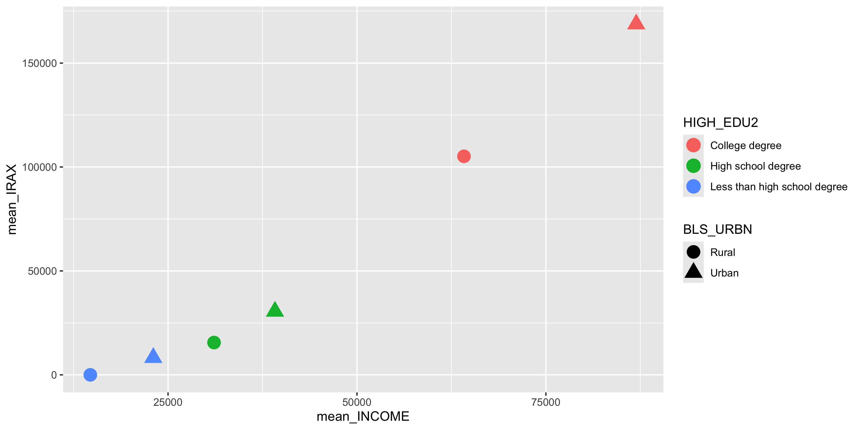
2 Urban 58987. 94512. 991Multiple Groupings
ce %>%
  group_by(BLS_URBN, HIGH_EDU2) %>%
  summarize(mean_INCOME = mean(INCOME, na.rm = TRUE),
            mean_IRAX = mean(IRAX, na.rm = TRUE),
            households = n()) %>%
  arrange(mean_IRAX)
# A tibble: 6 × 5
# Groups: BLS_URBN [2]
BLS_URBN HIGH_EDU2 mean_INCOME mean_IRAX households
<chr> <chr> <dbl> <dbl> <int>
1 Rural Less than high school degree 14715. 0 39
2 Urban Less than high school degree 23046. 8270. 381
3 Rural High school degree 31087. 15543. 192
4 Urban High school degree 39147. 30533. 2377
5 Rural College degree 64161. 105148. 118
6 Urban College degree 86957. 168767. 3194Piping into ggplot2
Naming Wrangled Data
When I make a new dataframe, what name should I give it? Importantly, should I write over my original dataframe or should I save a new dataframe?
- My answer:
- Is your new dataframe structurally different? If so, give it a new name.
- Are you removing values you will need for a future analysis within the same document? If so, give it a new name.
- Are you just adding to or cleaning the data? If so, then write over the original.
Sage Advice from ModernDive
“Crucial: Unless you are very confident in what you are doing, it is worthwhile not starting to code right away. Rather, first sketch out on paper all the necessary data wrangling steps not using exact code, but rather high-level pseudocode that is informal yet detailed enough to articulate what you are doing. This way you won’t confuse what you are trying to do (the algorithm) with how you are going to do it (writing dplyr code).”