Regression III: Categorical Predictors

Grayson White

Math 141
Week 4 | Fall 2025

Reminders

• Please fill out the Week 4 feedback survey (link in Slack)
• Lab 4 has other components besides the data collection we did in lab yesterday. Make sure to do the other questions and turn in by next Thurs!

Goals for Today

• Recap: Simple linear regression model
• Broadening our idea of linear regression

• Regression with a single, binary categorical explanatory variable
• Regression with a single categorical explanatory variable with more than 2 levels

Simple Linear Regression

Consider this model when:

• Response variable \((y)\): quantitative

• Explanatory variable \((x)\): quantitative

  • Have only ONE explanatory variable.

• AND, \(f()\) can be approximated by a line:

\[ \begin{align} y &= \beta_o + \beta_1 x + \epsilon \end{align} \]

Linear Regression

Linear regression is a flexible class of models that allow for:

• Both quantitative and categorical explanatory variables.

• Multiple explanatory variables.

• Curved relationships between the response variable and the explanatory variable.

• BUT the response variable is quantitative.

What About A Categorical Explanatory Variable?

• Response variable \((y)\): quantitative

• Have 1 categorical explanatory variable \((x)\) with two categories.

• Model form:

\[ \begin{align} y &= \beta_o + \beta_1 x + \epsilon \end{align} \]

• First, need to convert the categories of \(x\) to numbers.

Example: Halloween Candy

candy <- read_csv("https://raw.githubusercontent.com/fivethirtyeight/data/master/candy-power-ranking/candy-data.csv")
glimpse(candy)

Rows: 85
Columns: 13
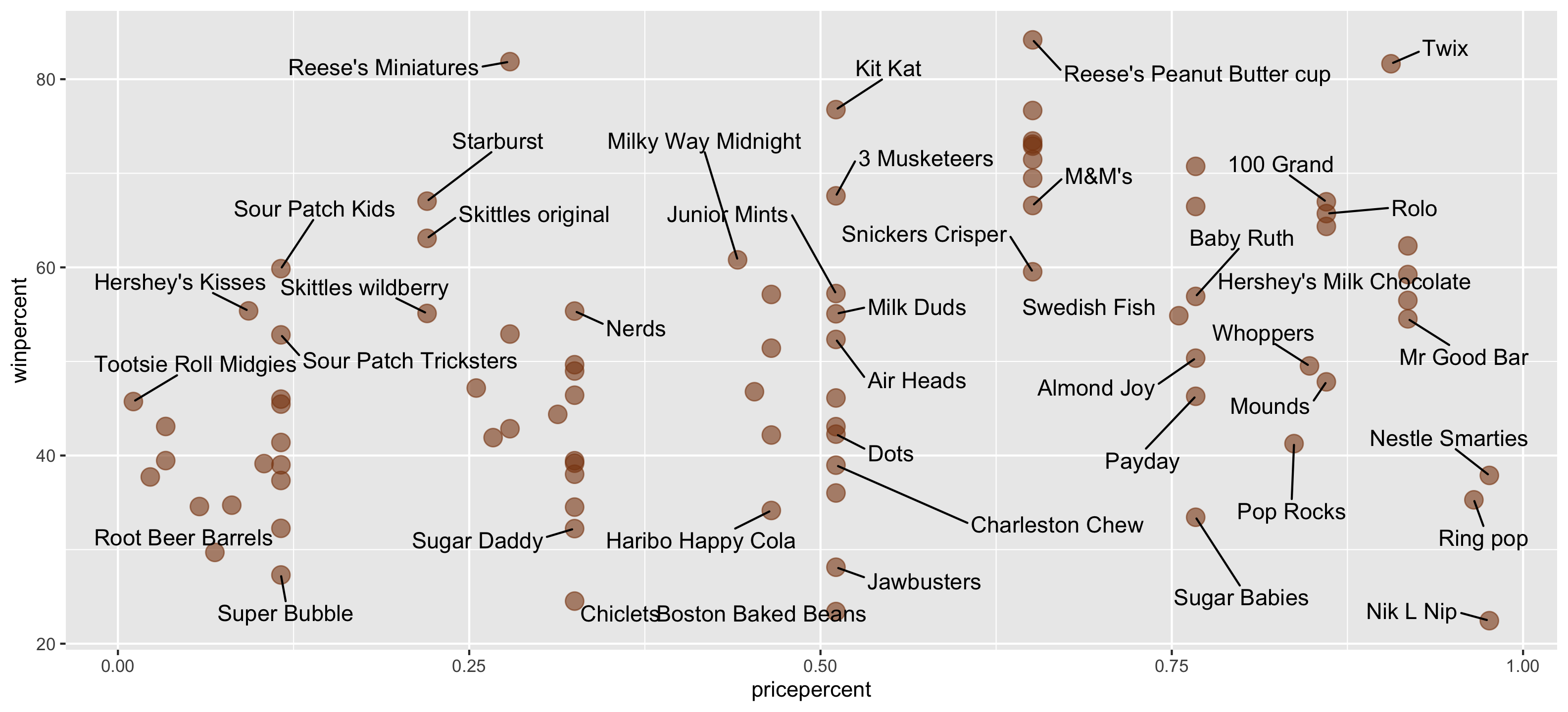
$ competitorname   <chr> "100 Grand", "3 Musketeers", "One dime", "One quarter…
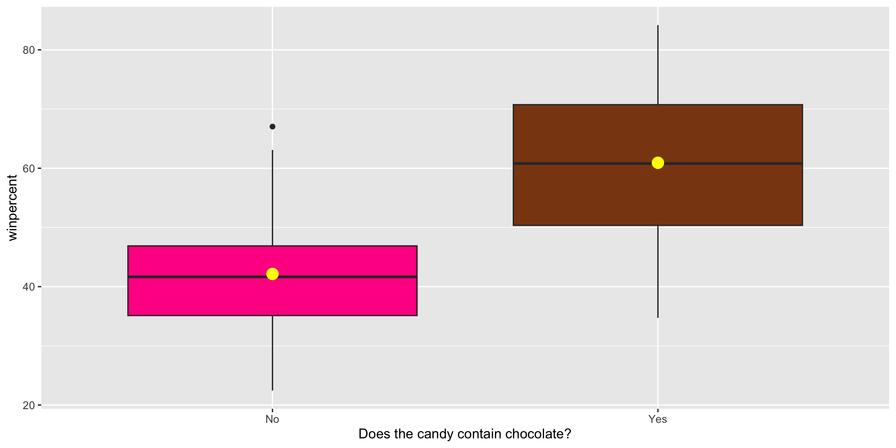
$ chocolate        <dbl> 1, 1, 0, 0, 0, 1, 1, 0, 0, 0, 1, 0, 0, 0, 0, 0, 0, 0,…
$ fruity           <dbl> 0, 0, 0, 0, 1, 0, 0, 0, 0, 1, 0, 1, 1, 1, 1, 1, 1, 1,…
$ caramel          <dbl> 1, 0, 0, 0, 0, 0, 1, 0, 0, 1, 0, 0, 0, 0, 0, 0, 0, 0,…
$ peanutyalmondy   <dbl> 0, 0, 0, 0, 0, 1, 1, 1, 0, 0, 0, 0, 0, 0, 0, 0, 0, 0,…
$ nougat           <dbl> 0, 1, 0, 0, 0, 0, 1, 0, 0, 0, 1, 0, 0, 0, 0, 0, 0, 0,…
$ crispedricewafer <dbl> 1, 0, 0, 0, 0, 0, 0, 0, 0, 0, 0, 0, 0, 0, 0, 0, 0, 0,…
$ hard             <dbl> 0, 0, 0, 0, 0, 0, 0, 0, 0, 0, 0, 0, 0, 0, 1, 0, 1, 1,…
$ bar              <dbl> 1, 1, 0, 0, 0, 1, 1, 0, 0, 0, 1, 0, 0, 0, 0, 0, 0, 0,…
$ pluribus         <dbl> 0, 0, 0, 0, 0, 0, 0, 1, 1, 0, 0, 1, 1, 1, 0, 1, 0, 1,…
$ sugarpercent     <dbl> 0.732, 0.604, 0.011, 0.011, 0.906, 0.465, 0.604, 0.31…
$ pricepercent     <dbl> 0.860, 0.511, 0.116, 0.511, 0.511, 0.767, 0.767, 0.51…
$ winpercent       <dbl> 66.97173, 67.60294, 32.26109, 46.11650, 52.34146, 50.…

What might be a good categorical explanatory variable of winpercent?

Exploratory Data Analysis

Before building the model, let’s explore and visualize the data!

• What dplyr functions should I use to find the mean and sd of winpercent by the categories of chocolate?

• What graph should we use to visualize the winpercent scores by chocolate?

Exploratory Data Analysis

# Summarize
candy %>%
  group_by(chocolate) %>%
  summarize(count = n(),
            mean_win = mean(winpercent), 
            sd_win = sd(winpercent))

# A tibble: 2 × 4
  chocolate count mean_win sd_win
      <dbl> <int>    <dbl>  <dbl>
1         0    48     42.1   10.2
2         1    37     60.9   12.8

Exploratory Data Analysis

ggplot(candy, aes(x = factor(chocolate), 
                   y = winpercent, 
                  fill = factor(chocolate))) +
  geom_boxplot() +
  stat_summary(fun = mean,
               geom = "point",
               color = "yellow",
               size = 4) +
  guides(fill = "none") +
  scale_fill_manual(values =
                      c("0" = "deeppink",
                        "1" = "chocolate4")) +
  scale_x_discrete(labels = c("No", "Yes"),
                   name =
          "Does the candy contain chocolate?")

Exploratory Data Analysis

ggplot(candy, aes(x = factor(chocolate), 
                   y = winpercent, 
                  fill = factor(chocolate))) +
  geom_boxplot() +
  stat_summary(fun = mean,
               geom = "point",
               color = "yellow",
               size = 4) +
  guides(fill = "none") +
  scale_fill_manual(values =
                      c("0" = "deeppink",
                        "1" = "chocolate4")) +
  scale_x_discrete(labels = c("No", "Yes"),
                   name =
          "Does the candy contain chocolate?")

Exploratory Data Analysis

ggplot(candy, aes(x = factor(chocolate), 
                   y = winpercent, 
                  fill = factor(chocolate))) +
  geom_boxplot() +
  stat_summary(fun = mean,
               geom = "point",
               color = "yellow",
               size = 4) +
  guides(fill = "none") +
  scale_fill_manual(values =
                      c("0" = "deeppink",
                        "1" = "chocolate4")) +
  scale_x_discrete(labels = c("No", "Yes"),
                   name =
          "Does the candy contain chocolate?")

Exploratory Data Analysis

ggplot(candy, aes(x = factor(chocolate), 
                   y = winpercent, 
                  fill = factor(chocolate))) +
  geom_boxplot() +
  stat_summary(fun = mean,
               geom = "point",
               color = "yellow",
               size = 4) +
  guides(fill = "none") +
  scale_fill_manual(values =
                      c("0" = "deeppink",
                        "1" = "chocolate4")) +
  scale_x_discrete(labels = c("No", "Yes"),
                   name =
          "Does the candy contain chocolate?")

Exploratory Data Analysis

ggplot(candy, aes(x = factor(chocolate), 
                   y = winpercent, 
                  fill = factor(chocolate))) +
  geom_boxplot() +
  stat_summary(fun = mean,
               geom = "point",
               color = "yellow",
               size = 4) +
  guides(fill = "none") +
  scale_fill_manual(values =
                      c("0" = "deeppink",
                        "1" = "chocolate4")) +
  scale_x_discrete(labels = c("No", "Yes"),
                   name =
          "Does the candy contain chocolate?")

Exploratory Data Analysis

ggplot(candy, aes(x = factor(chocolate), 
                   y = winpercent, 
                  fill = factor(chocolate))) +
  geom_boxplot() +
  stat_summary(fun = mean,
               geom = "point",
               color = "yellow",
               size = 4) +
  guides(fill = "none") +
  scale_fill_manual(values =
                      c("0" = "deeppink",
                        "1" = "chocolate4")) +
  scale_x_discrete(labels = c("No", "Yes"),
                   name =
          "Does the candy contain chocolate?")

Fit the Linear Regression Model

Model Form:

\[ \begin{align} y &= \beta_o + \beta_1 x + \epsilon \end{align} \]

When \(x = 0\):

When \(x = 1\):

mod <- lm(winpercent ~ chocolate, data = candy)
library(moderndive)
get_regression_table(mod)

# A tibble: 2 × 7
  term      estimate std_error statistic p_value lower_ci upper_ci
  <chr>        <dbl>     <dbl>     <dbl>   <dbl>    <dbl>    <dbl>
1 intercept     42.1      1.65     25.6        0     38.9     45.4
2 chocolate     18.8      2.50      7.52       0     13.8     23.7

Notes

• When the explanatory variable is categorical, \(\beta_o\) and \(\beta_1\) no longer represent the intercept and slope.

• Now \(\beta_o\) represents the (population) mean of the response variable when \(x = 0\).

• And, \(\beta_1\) represents the change in the (population) mean response going from \(x = 0\) to \(x = 1\).

• Can also do prediction:

new_candy <- data.frame(chocolate = c(0, 1))
predict(mod, newdata = new_candy)

       1        2 
42.14226 60.92153 

Turns Out Reese’s Miniatures Are Under-Priced…

New example: Palmer Penguins

library(palmerpenguins)

Take a look at the data

glimpse(penguins)

Rows: 344
Columns: 8
$ species           <fct> Adelie, Adelie, Adelie, Adelie, Adelie, Adelie, Adel…
$ island            <fct> Torgersen, Torgersen, Torgersen, Torgersen, Torgerse…
$ bill_length_mm    <dbl> 39.1, 39.5, 40.3, NA, 36.7, 39.3, 38.9, 39.2, 34.1, …
$ bill_depth_mm     <dbl> 18.7, 17.4, 18.0, NA, 19.3, 20.6, 17.8, 19.6, 18.1, …
$ flipper_length_mm <int> 181, 186, 195, NA, 193, 190, 181, 195, 193, 190, 186…
$ body_mass_g       <int> 3750, 3800, 3250, NA, 3450, 3650, 3625, 4675, 3475, …
$ sex               <fct> male, female, female, NA, female, male, female, male…
$ year              <int> 2007, 2007, 2007, 2007, 2007, 2007, 2007, 2007, 2007…

We’d like to predict a penguin’s bill length based on their species.

Response variable?

Explanatory variable?

Exploratory data analysis

penguins %>%
  group_by(species) %>%
  summarize(
    avg_bill_length = mean(bill_length_mm,
                           na.rm = TRUE)
    )

# A tibble: 3 × 2
  species   avg_bill_length
  <fct>               <dbl>
1 Adelie               38.8
2 Chinstrap            48.8
3 Gentoo               47.5

ggplot(penguins, 
       aes(x = species,
           y = bill_length_mm, 
           fill = species)) +
  geom_boxplot() +
  scale_fill_manual(values = c("steelblue",
                               "goldenrod", 
                               "plum3")) +
  guides(fill = "none") +
  theme_bw()

How do we handle more than 2 groups???

Boardwork

Fit the model in R

\[ y = \beta_o + \beta_1 x_{species:Chinstrap} + \beta_2 x_{species:Gentoo} + \epsilon \]

penguin_mod <- lm(bill_length_mm ~ species, penguins)
get_regression_table(penguin_mod)

# A tibble: 3 × 7
  term               estimate std_error statistic p_value lower_ci upper_ci
  <chr>                 <dbl>     <dbl>     <dbl>   <dbl>    <dbl>    <dbl>
1 intercept             38.8      0.241     161.        0    38.3     39.3 
2 species: Chinstrap    10.0      0.432      23.2       0     9.19    10.9 
3 species: Gentoo        8.71     0.36       24.2       0     8.01     9.42

\[\begin{align*} \hat{y} &= \hat{\beta}_o + \hat{\beta}_1 \cdot x_{species:Chinstrap} + \hat{\beta}_2 \cdot x_{species:Gentoo} \\ &= 38.8 + 10.0 \cdot x_{species:Chinstrap} + 8.71 \cdot x_{species:Gentoo} \end{align*}\]

Coefficient interpretation?

Remember to diagnose your models!

library(gglm)
ggplot(penguin_mod) +
  stat_fitted_resid()

Remember to diagnose your models!

ggplot(penguin_mod) +
  stat_resid_hist()

ggplot(penguin_mod) +
  stat_normal_qq()

Multiple Linear Regression: A peak into next week

Recall our penguin model

\[ y = \beta_o + \beta_1 x_{species:Chinstrap} + \beta_2 x_{species:Gentoo} + \epsilon \]

Even though we are using one predictor (species), we now have \(\beta_o,~ \beta_1,\) and \(\beta_2\)!

• We recoded the species predictor into two binary predictors.
• We are actually doing multiple linear regression now
• Next time: We’ll formalize and extend multiple linear regression