We need to be precise and careful when interpreting estimated coefficients!
Intercept: We expect/predict\(y\) to be \(\hat{\beta}_o\)on average when \(x = 0\).
Slope: For a one-unit increase in \(x\), we expect/predict\(y\) to change by \(\hat{\beta}_1\) units on average.
These interpretations are non-specific to the context of our model, but when we are interpreting coefficients, we always need to interpret the coefficients in context
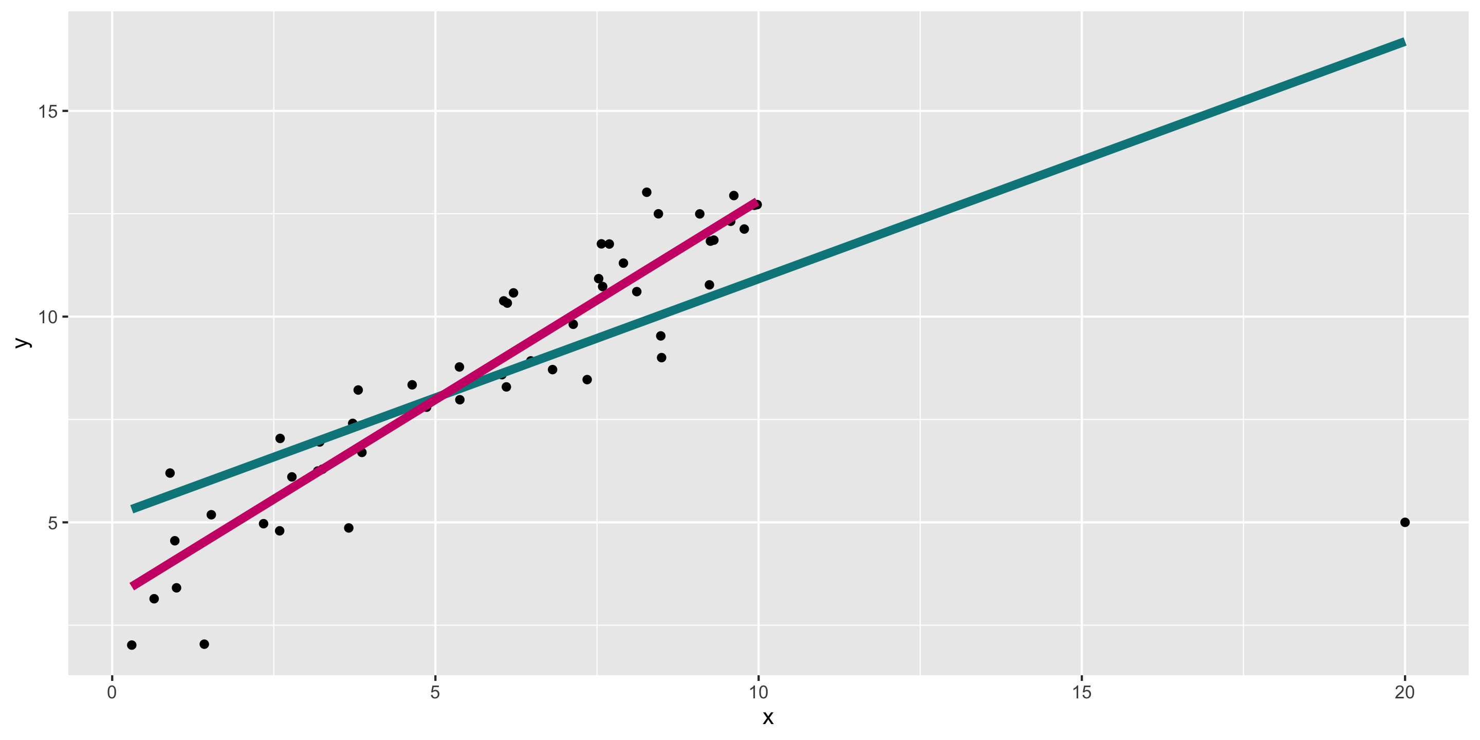
We can always find the line of best fit to explore data, but…
To make accurate predictions or inferences, certain conditions should be met.
To responsibly use linear regression tools for prediction or inference, we require:
Linearity: The relationship between explanatory and response variables must be approximately linear
Check using scatterplot of data, or residual plot
Independence: The observations should be independent of one another.
Can check by considering data context, and
by looking at residual scatterplots too
Normality: The distribution of residuals should be approximately bell-shaped, unimodal, symmetric, and centered at 0 at every “slice” of the explanatory variable
Simple check: look at histogram of residuals
Better to use a “Q-Q plot”
Equal Variability: Variance of residuals should be roughly constant across data set. Also called “homoscedasticity”. Models that violate this assumption are sometimes called “heteroscedastic”
Check using residual plot.
A cute way to remember this: “LINE”
Linearity
Independence
Normality
Equal Variability
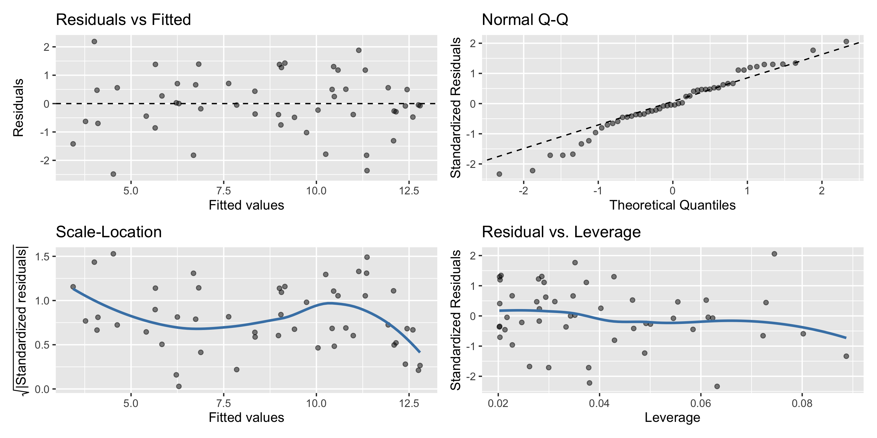
Assessing conditions: diagnostics plots
In order to assess if we’ve met the described conditions, we will utilize four common diagnostics plots:
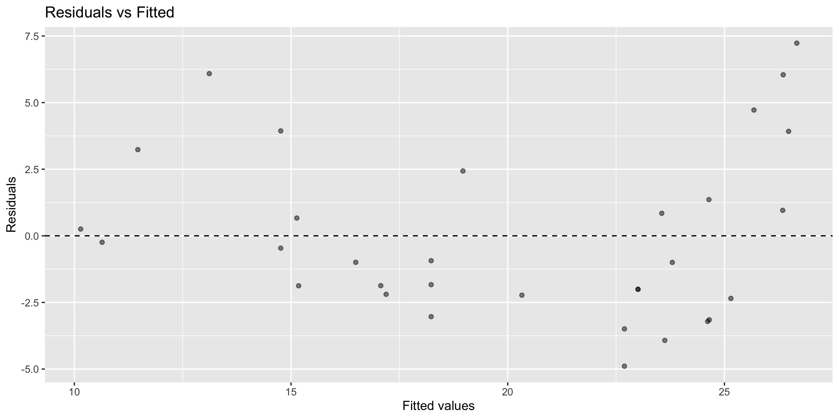
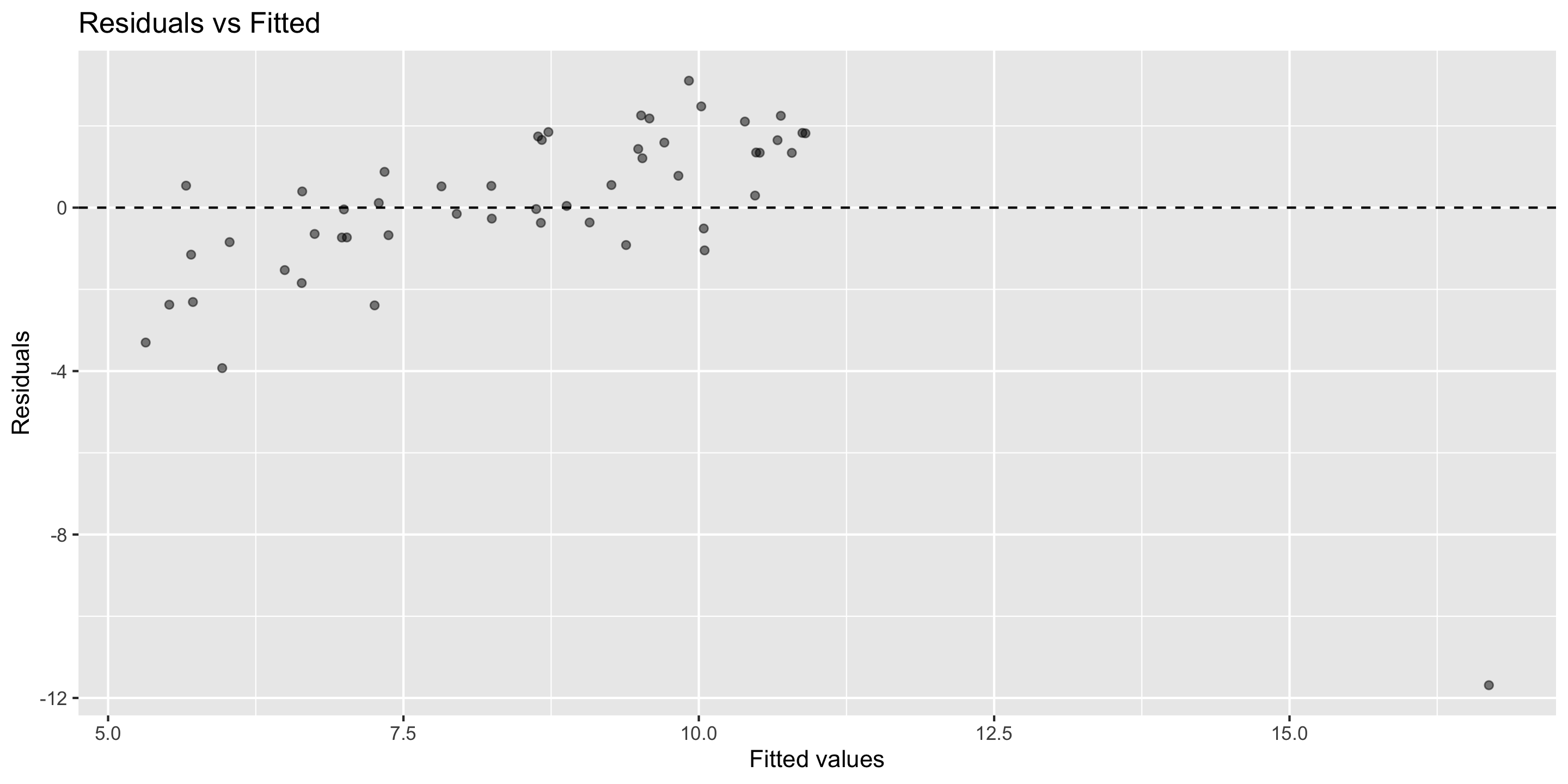
Residual vs. fitted plot (i.e. ‘residual plot’)
for assessing linearity, independence, and equal variability
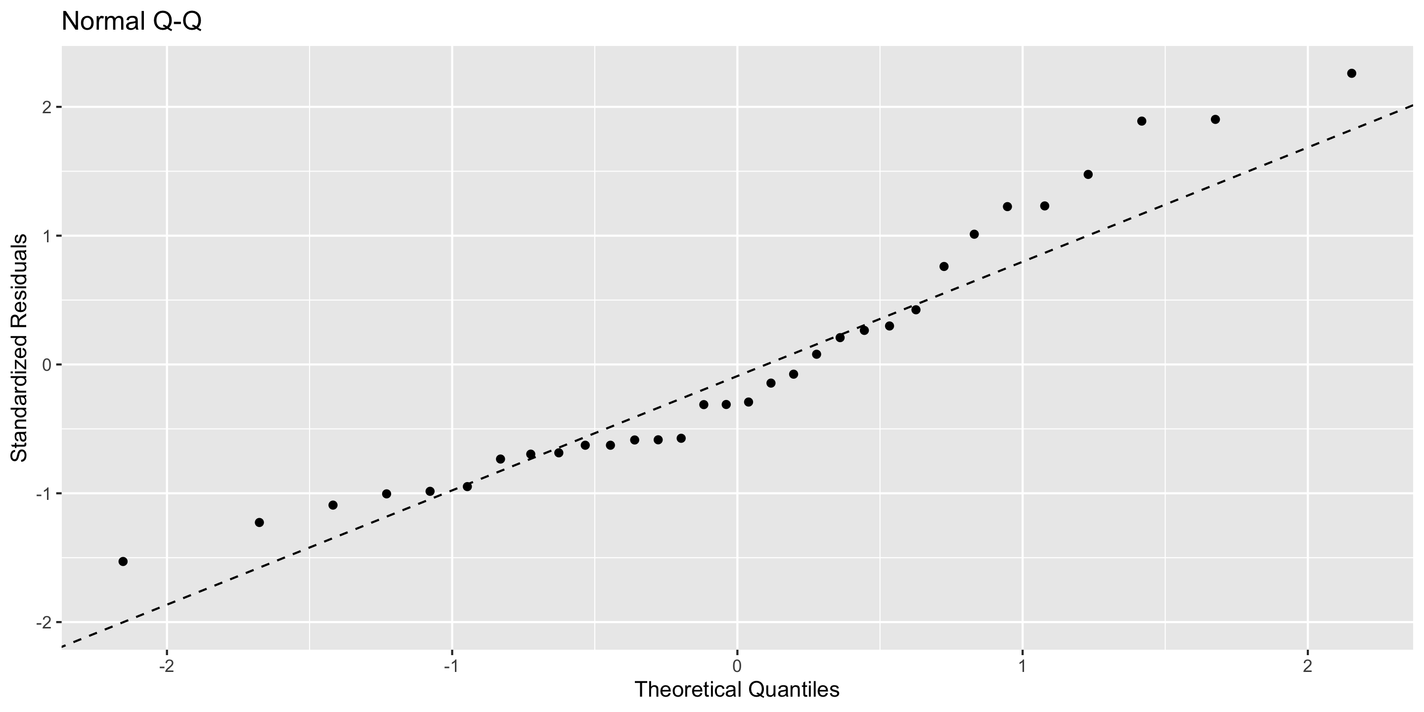
Normal Q-Q plot
for assessing normality
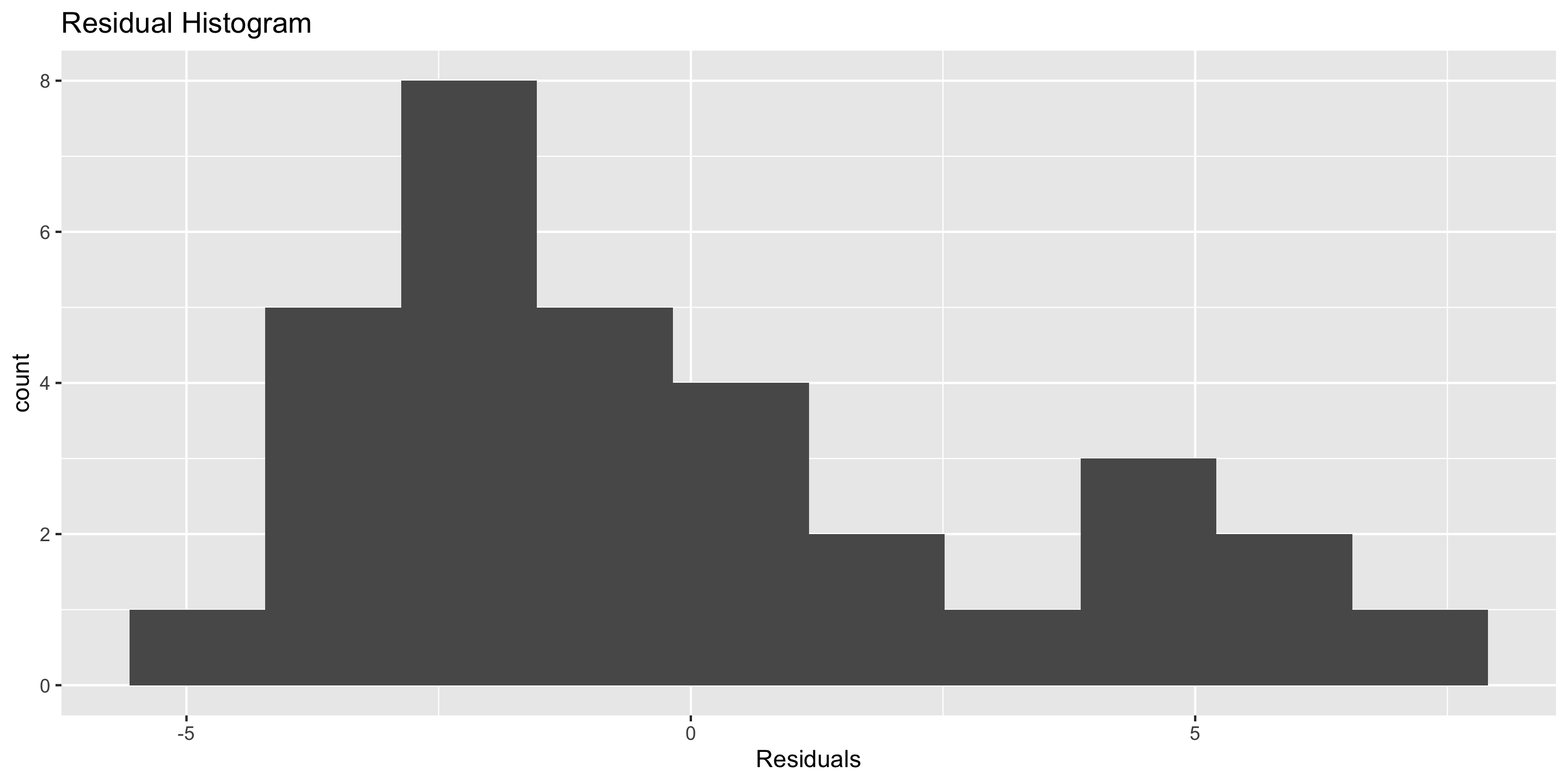
Residual histogram
for assessing normality
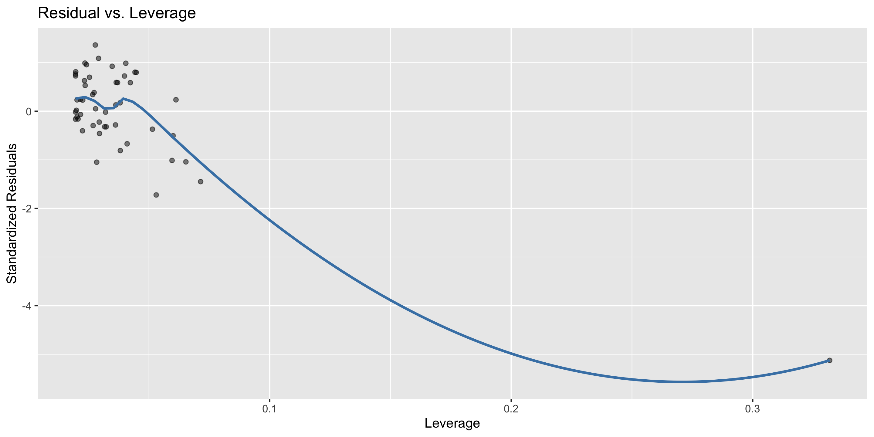
Residual vs. leverage plot
for assessing the influence of outliers
In order to make these plots, we’ll use the gglm (grammer of graphics for linear model diagnostics) package.
# Run the below code (without the '#') once# install.packages("gglm") # Then load with:library(gglm)
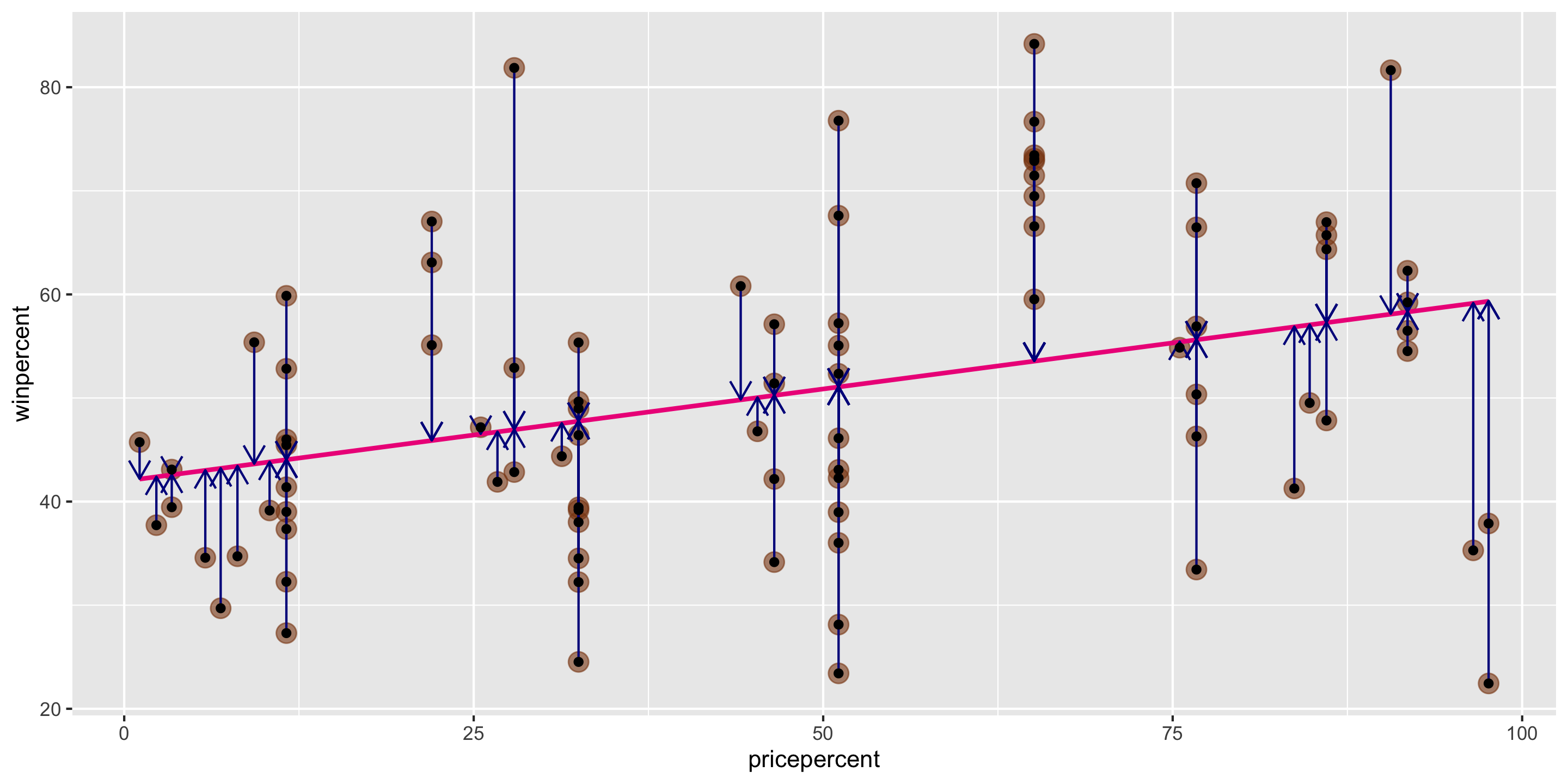
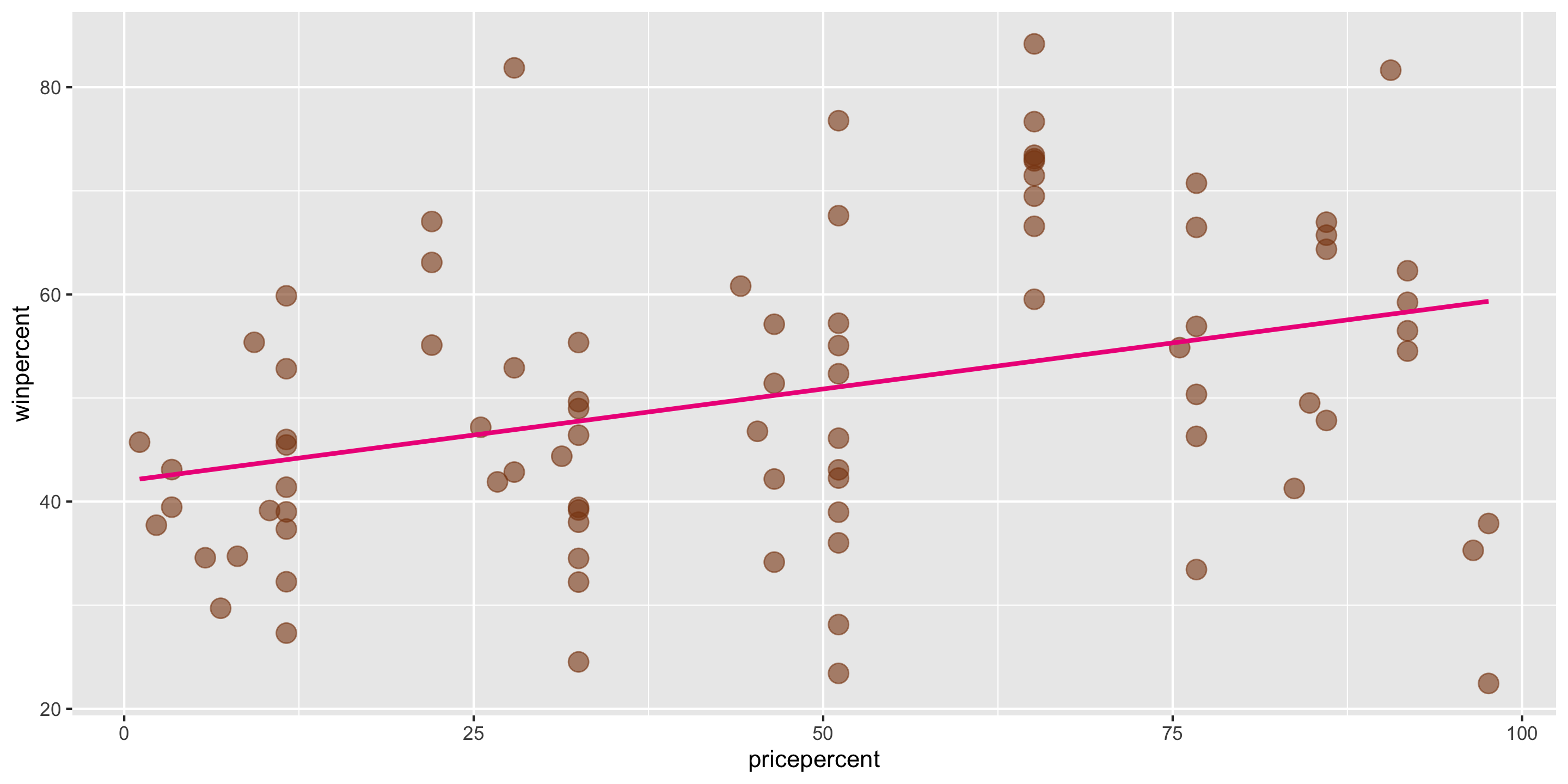
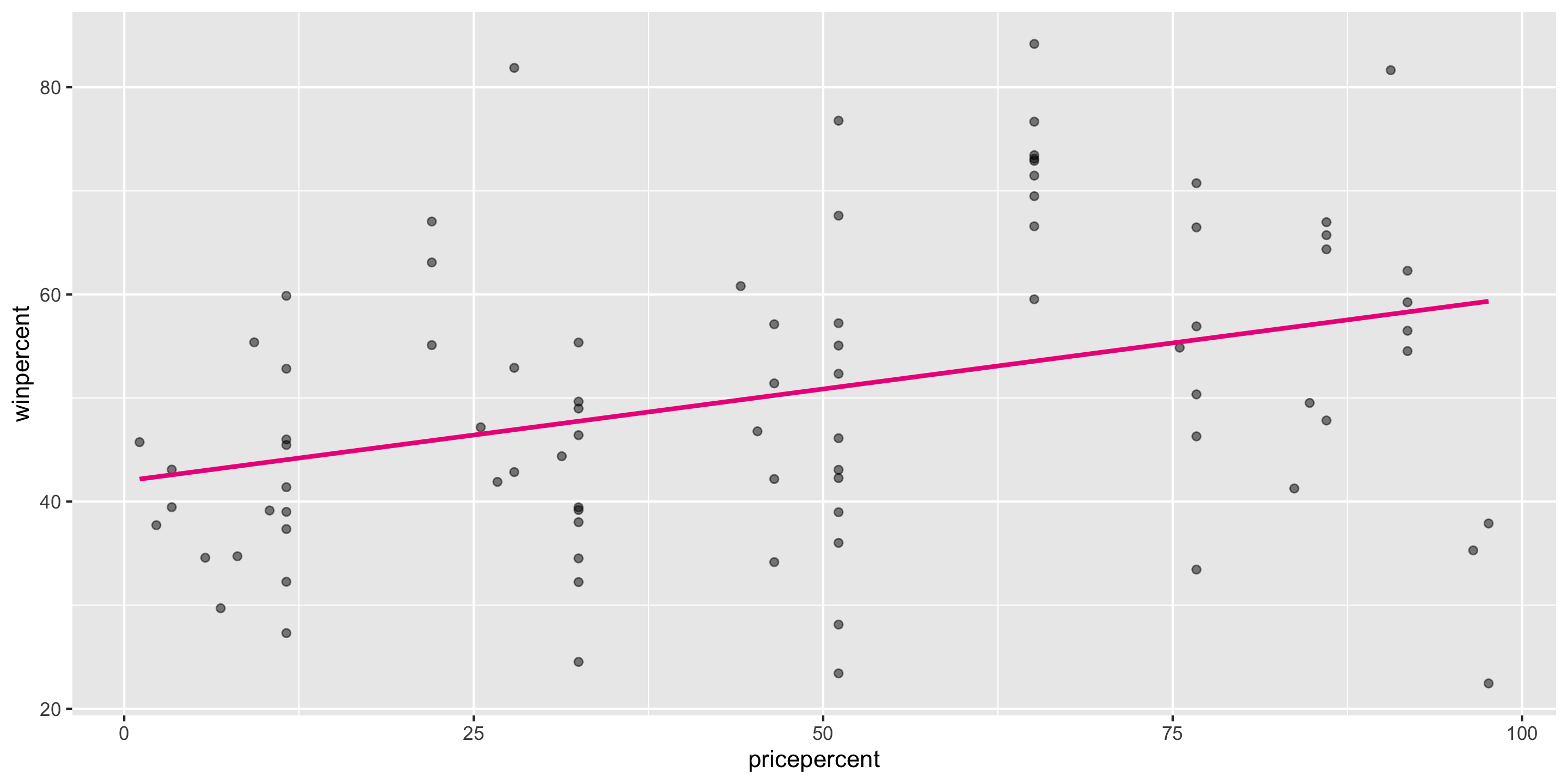
Recall out simple linear regression model
mod <-lm(winpercent ~ pricepercent, data = candy)
Let’s check if this meets the LINE assumptions
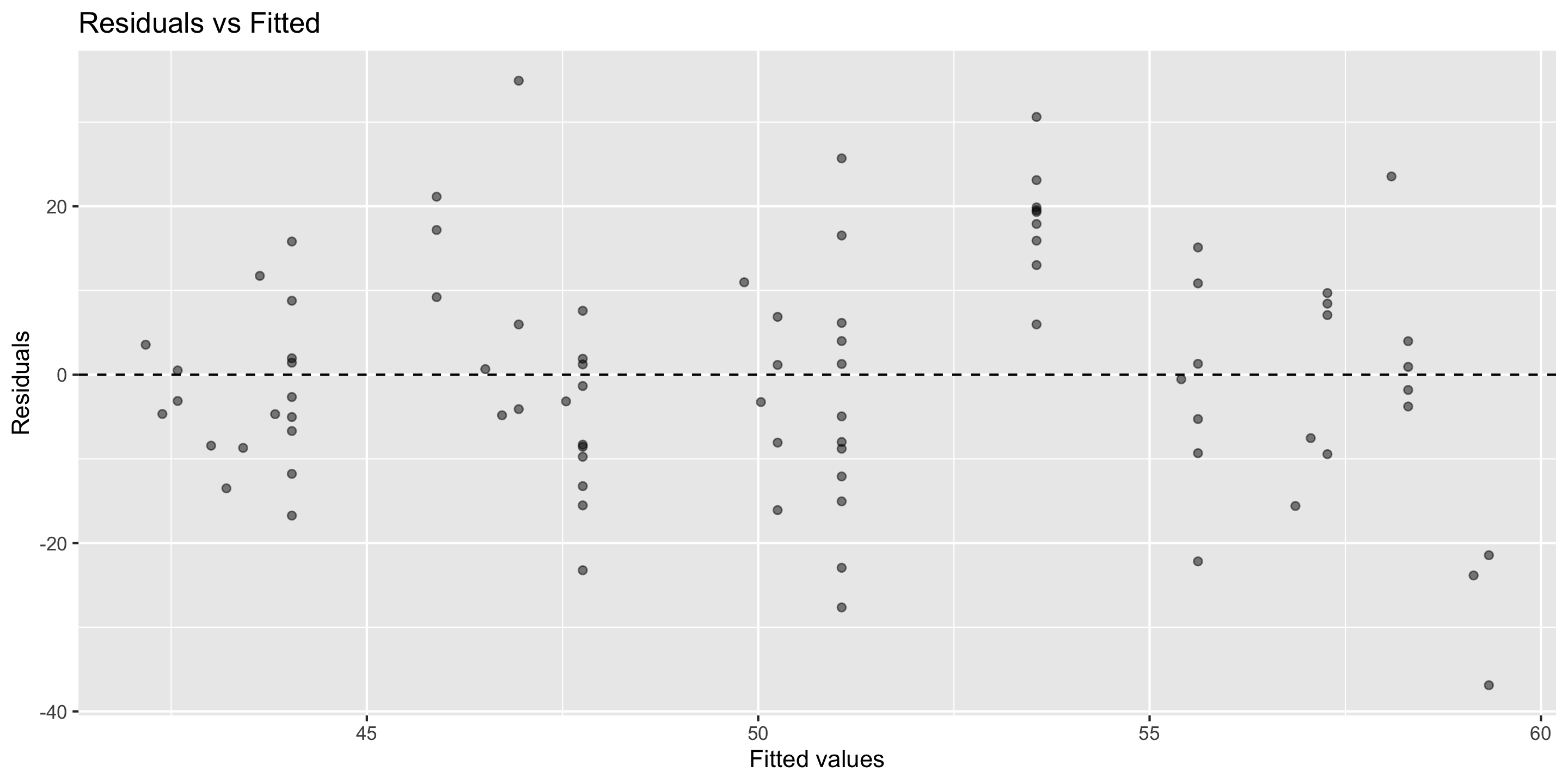
Residual vs. fitted plot
ggplot(mod) +stat_fitted_resid()
Linearity: ✅
Independence: ✅
Equal Variability: ✅
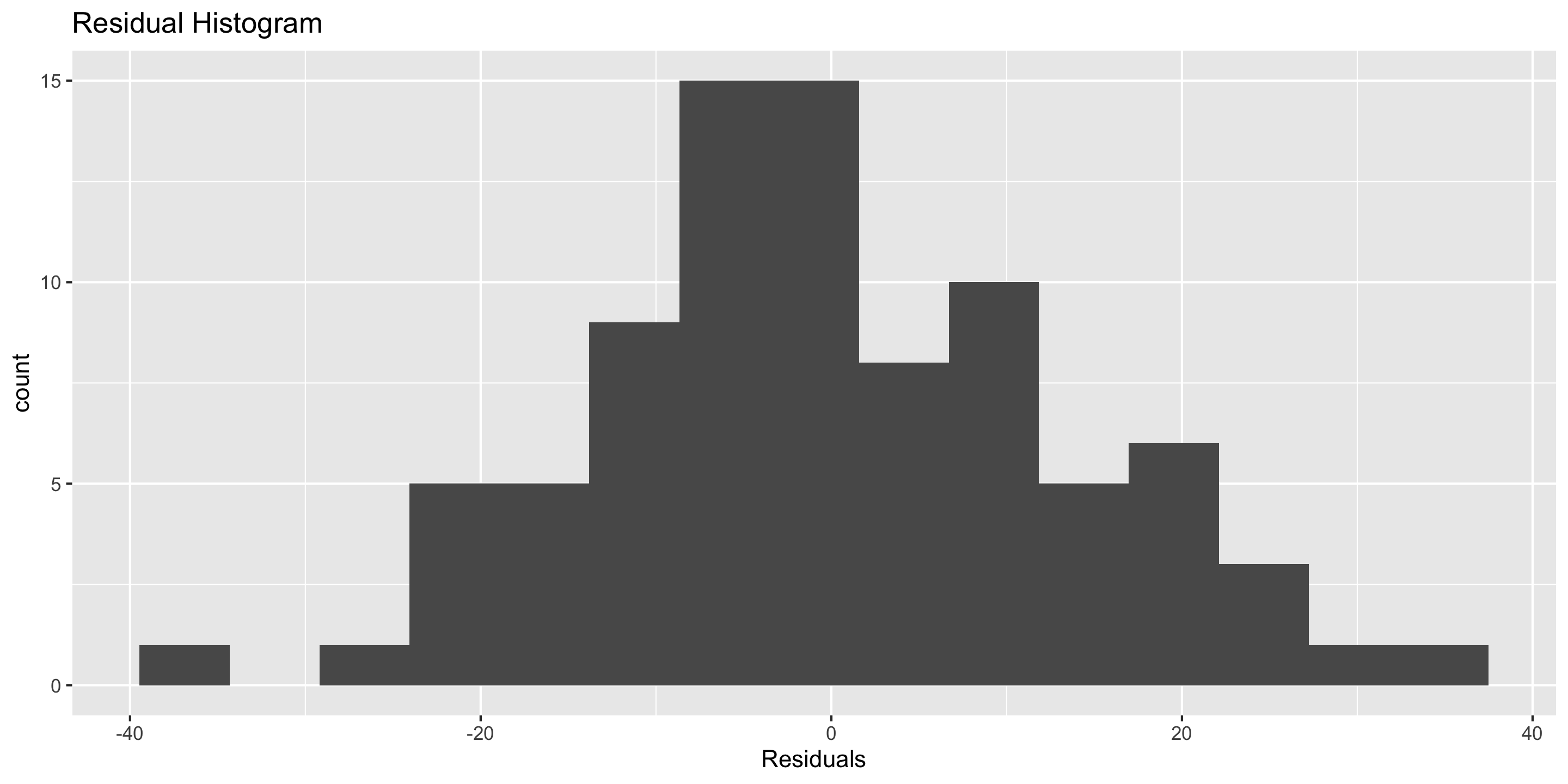
Checking normality: residual histogram
ggplot(mod) +stat_resid_hist(bins =15)
Normality: 🤔
Looks pretty good!
We’ll look at a Q-Q plot to further assess!
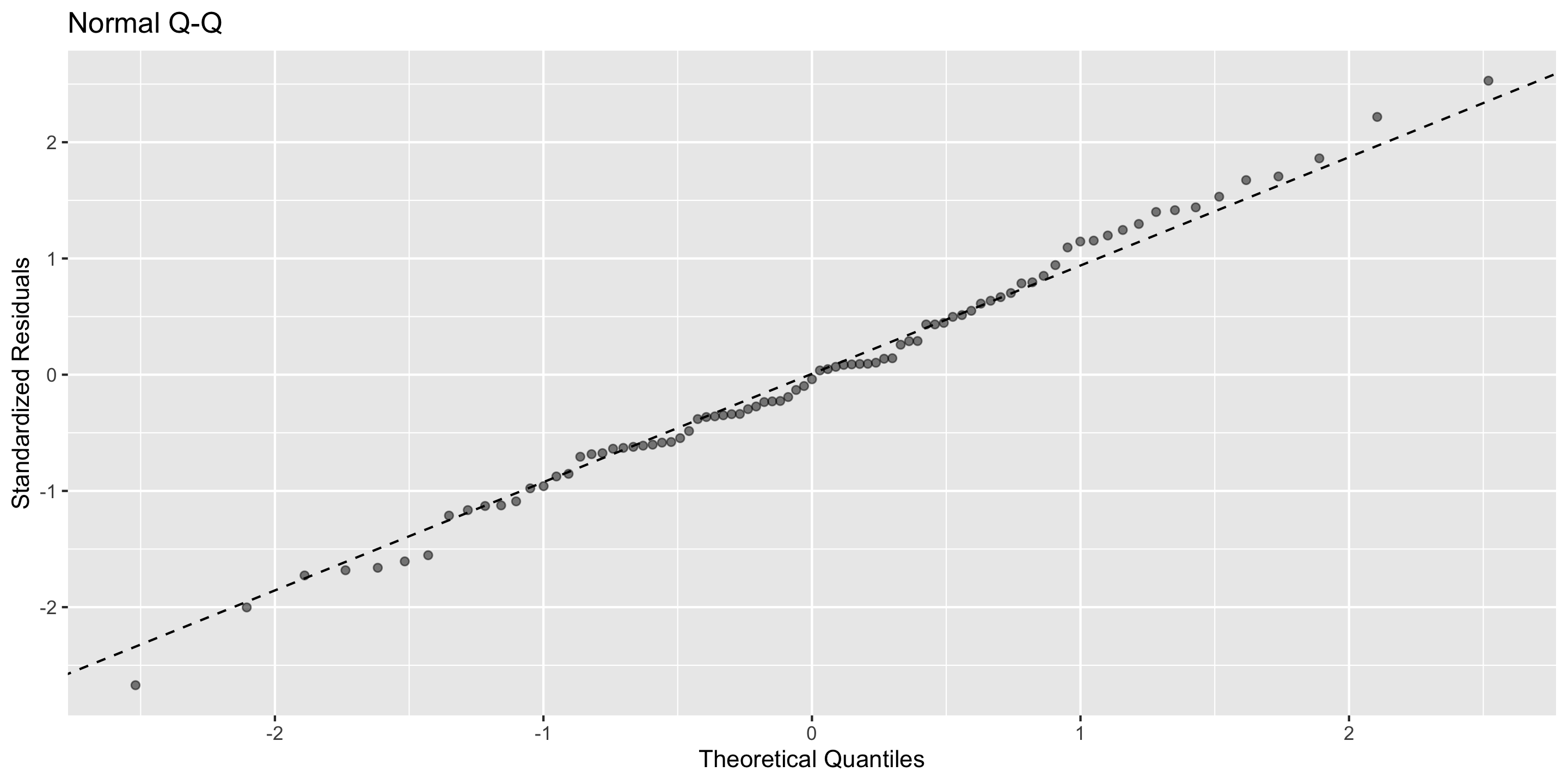
Checking normality: Q-Q plot
ggplot(mod) +stat_normal_qq()
Normality: ✅
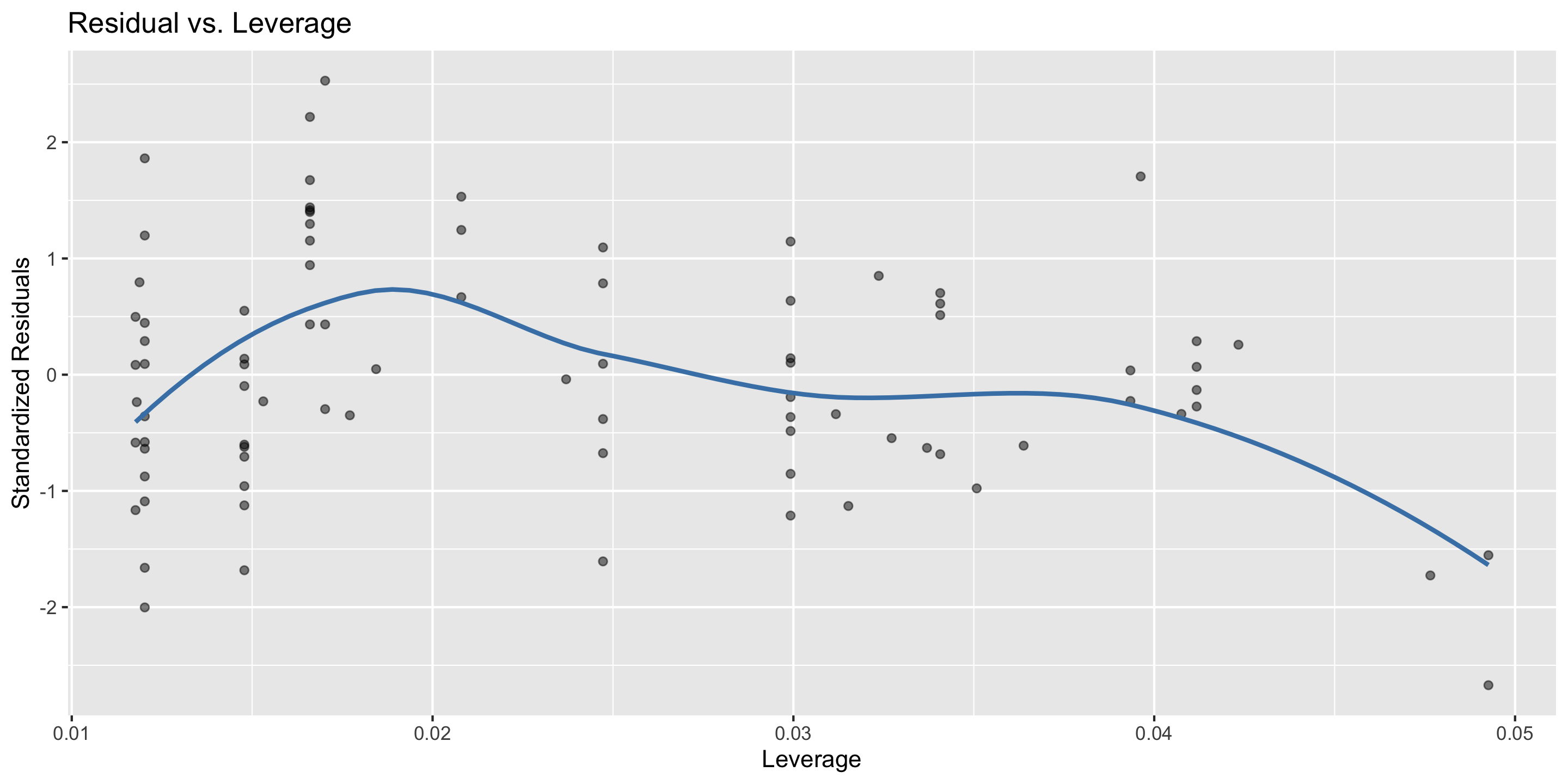
Checking outliers: Residuals vs. leverage plot
ggplot(mod) +stat_resid_leverage()
Looks pretty good! 🤩
Now let’s look at some models that violate these assumptions…
New model
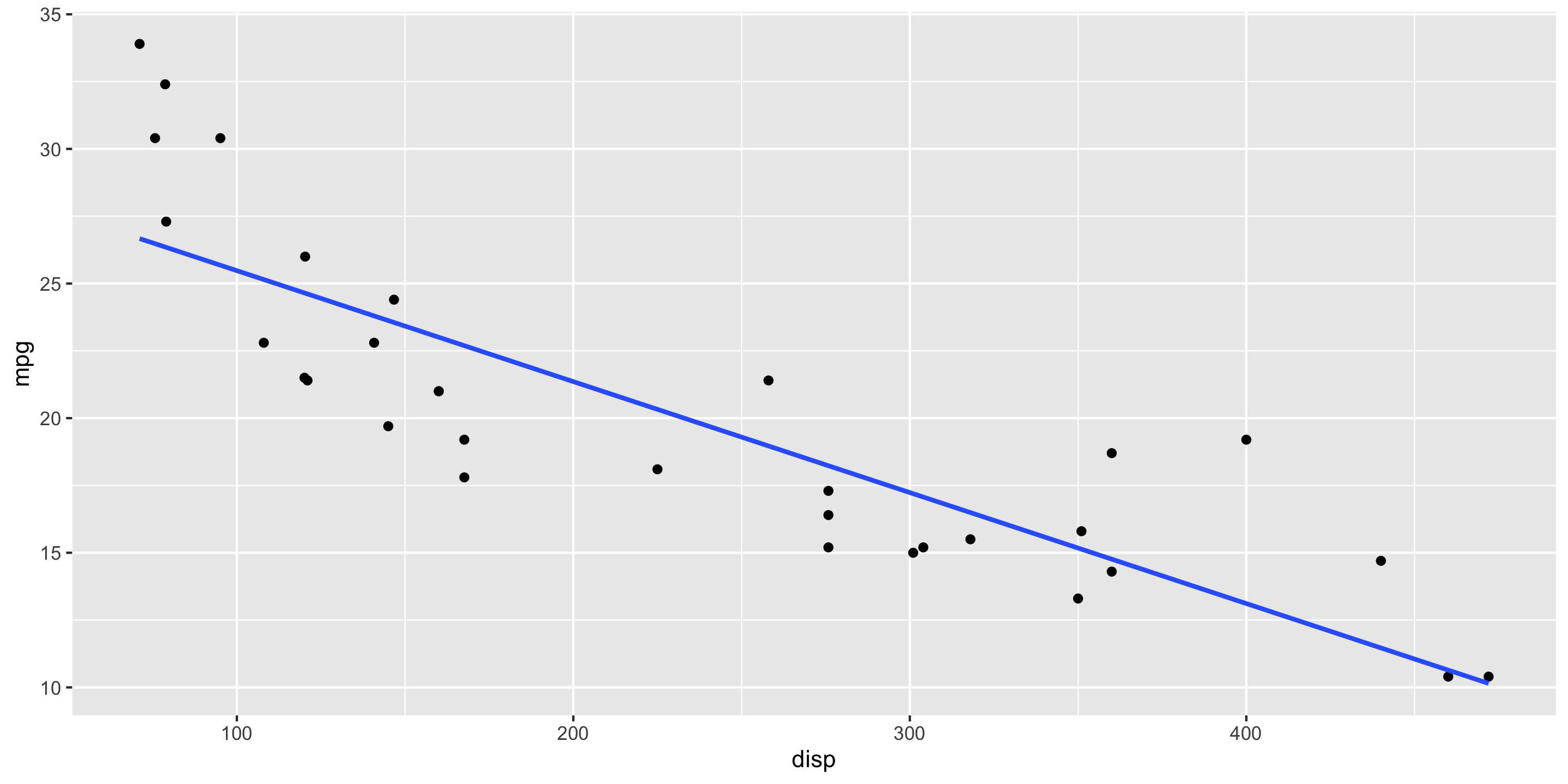
Predicting miles per gallon from engine displacement
data(mtcars)ggplot(mtcars, aes(x = disp, y = mpg)) +geom_point() +geom_smooth(method ="lm", se =FALSE)
New model
mpg_mod <-lm(formula = mpg ~ disp, data = mtcars)get_regression_table(mpg_mod)