
Model Guidance
Grayson White
Math 141
Week 5 | Fall 2025
Model Building Guidance
Shouldn’t we always include the interaction term?
Guiding Principle: Occam’s Razor for Modeling
“All other things being equal, simpler models are to be preferred over complex ones.” – ModernDive
Guiding Principle: Consider your modeling goals.
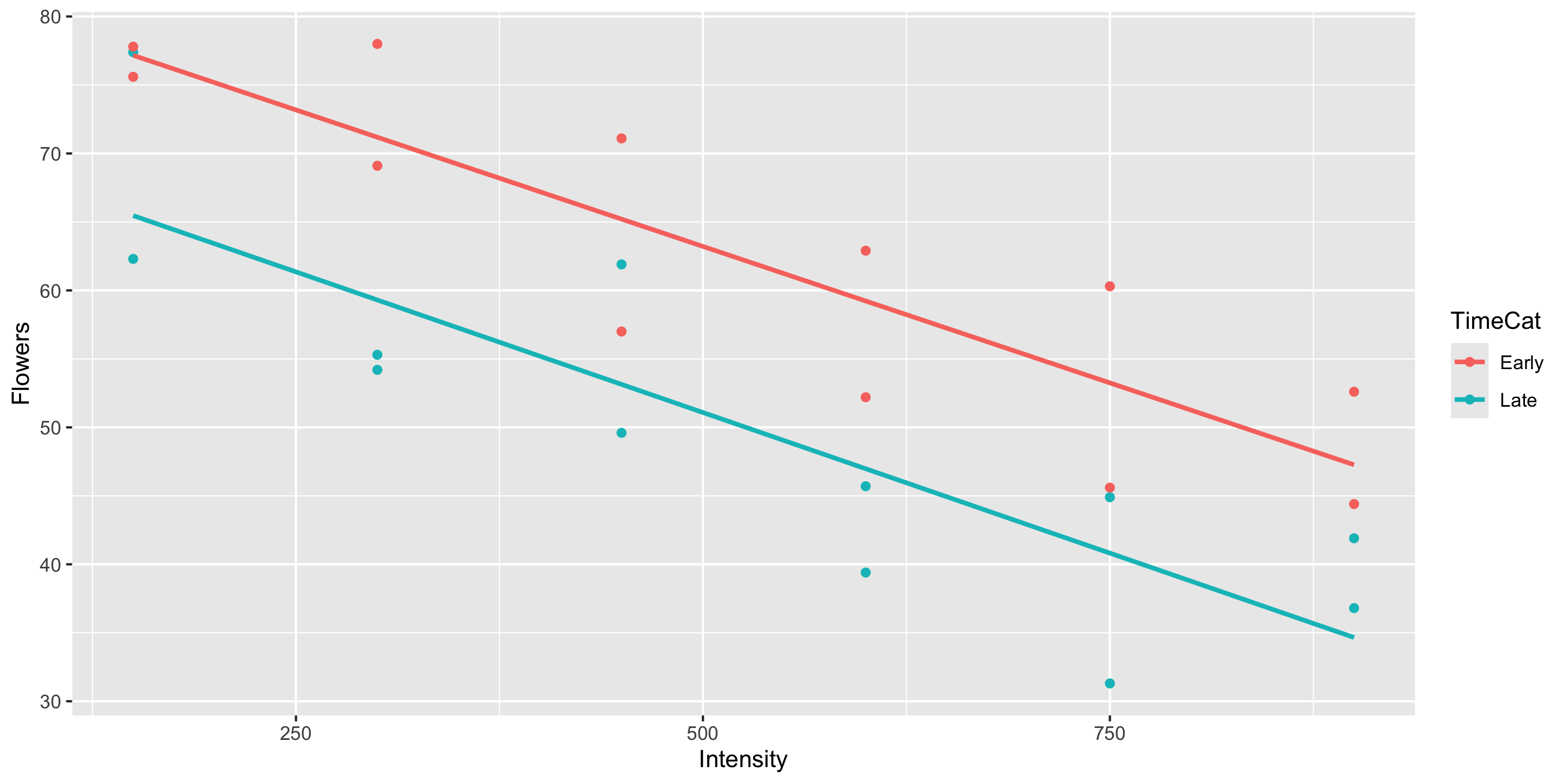
- The equal slopes model allows us to control for the intensity of the light and then see the impact of being in the early or late timing groups on the number of flowers.
- Later in the course will learn statistical procedures for determining whether or not a particular term should be included in the model.
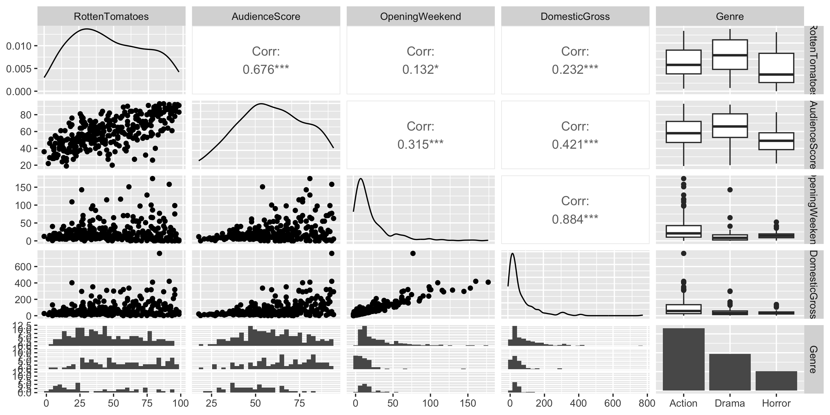
Example: Movie Ratings
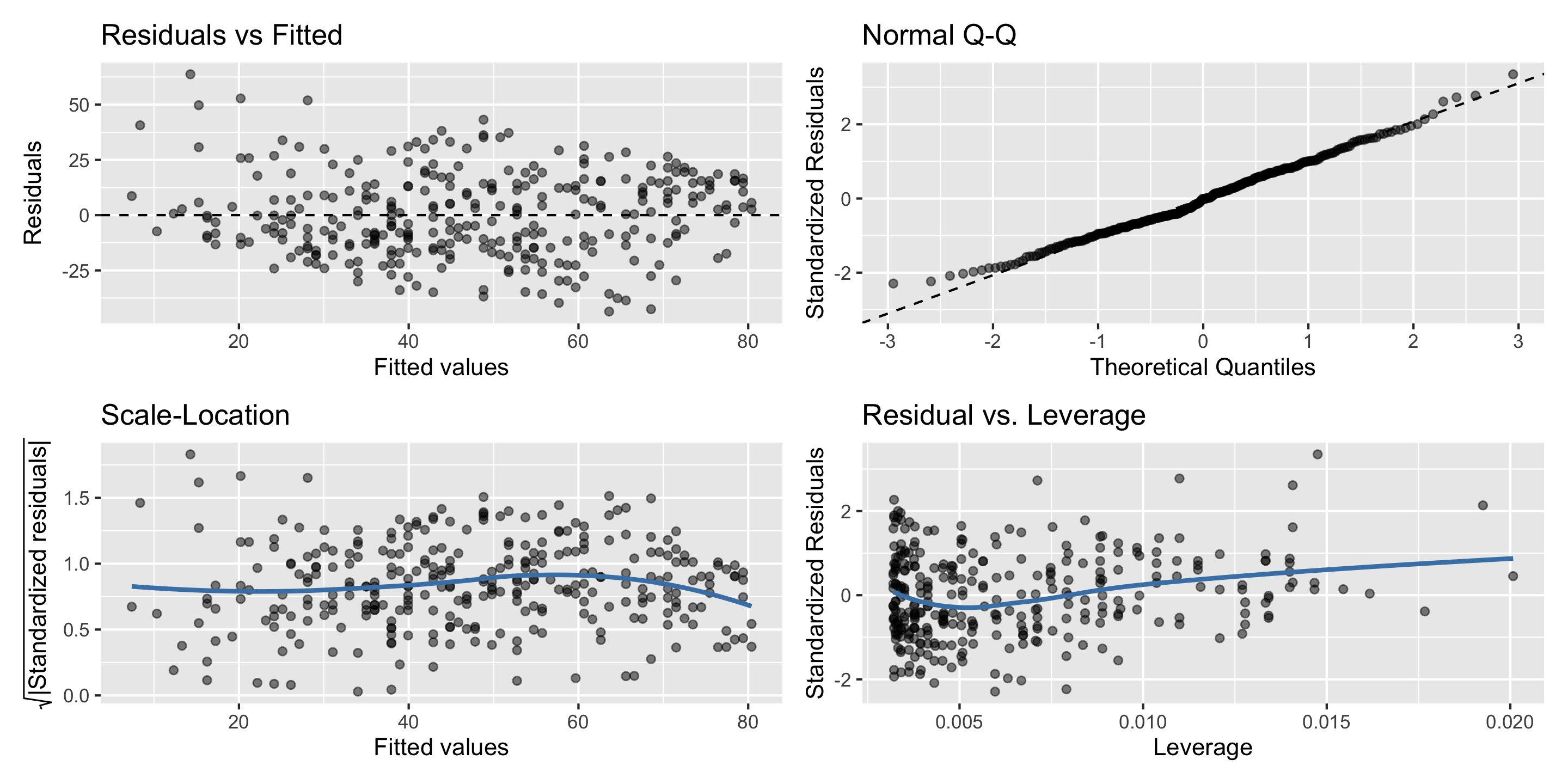
Model Building Guidance: Diagnostic Plots
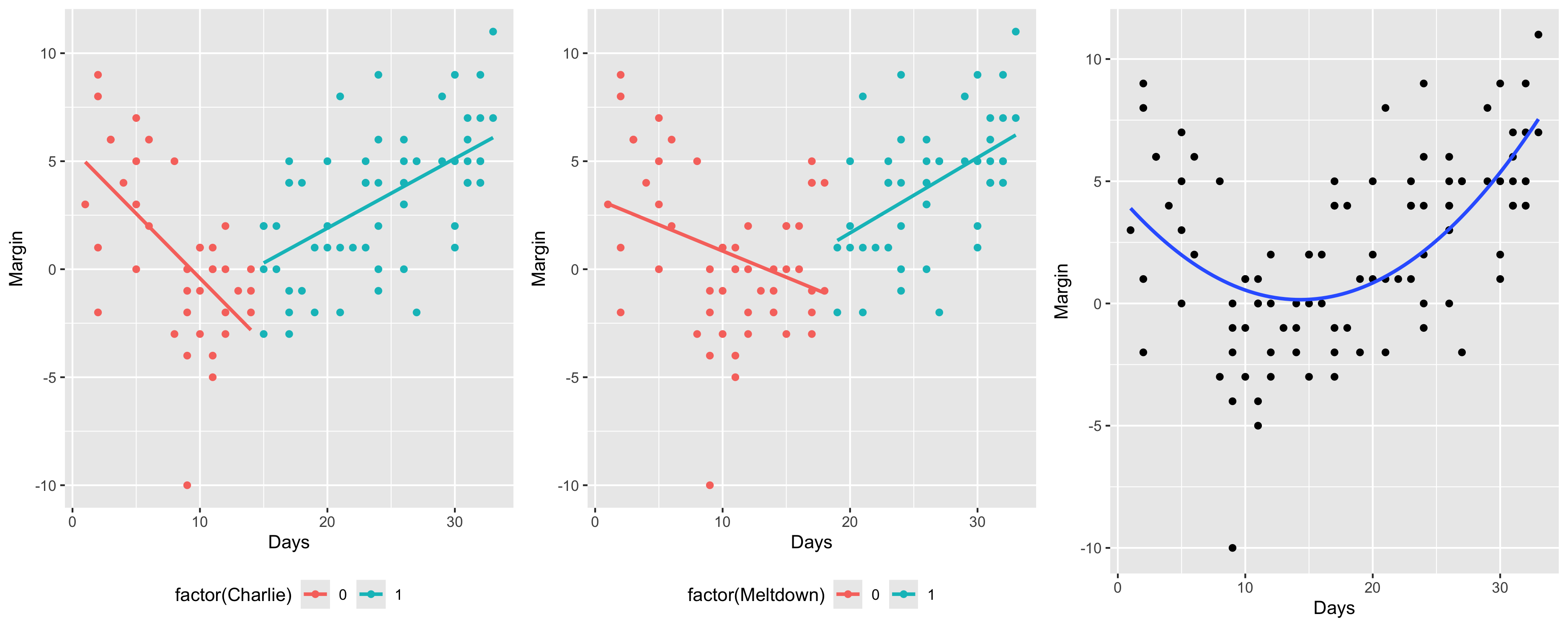
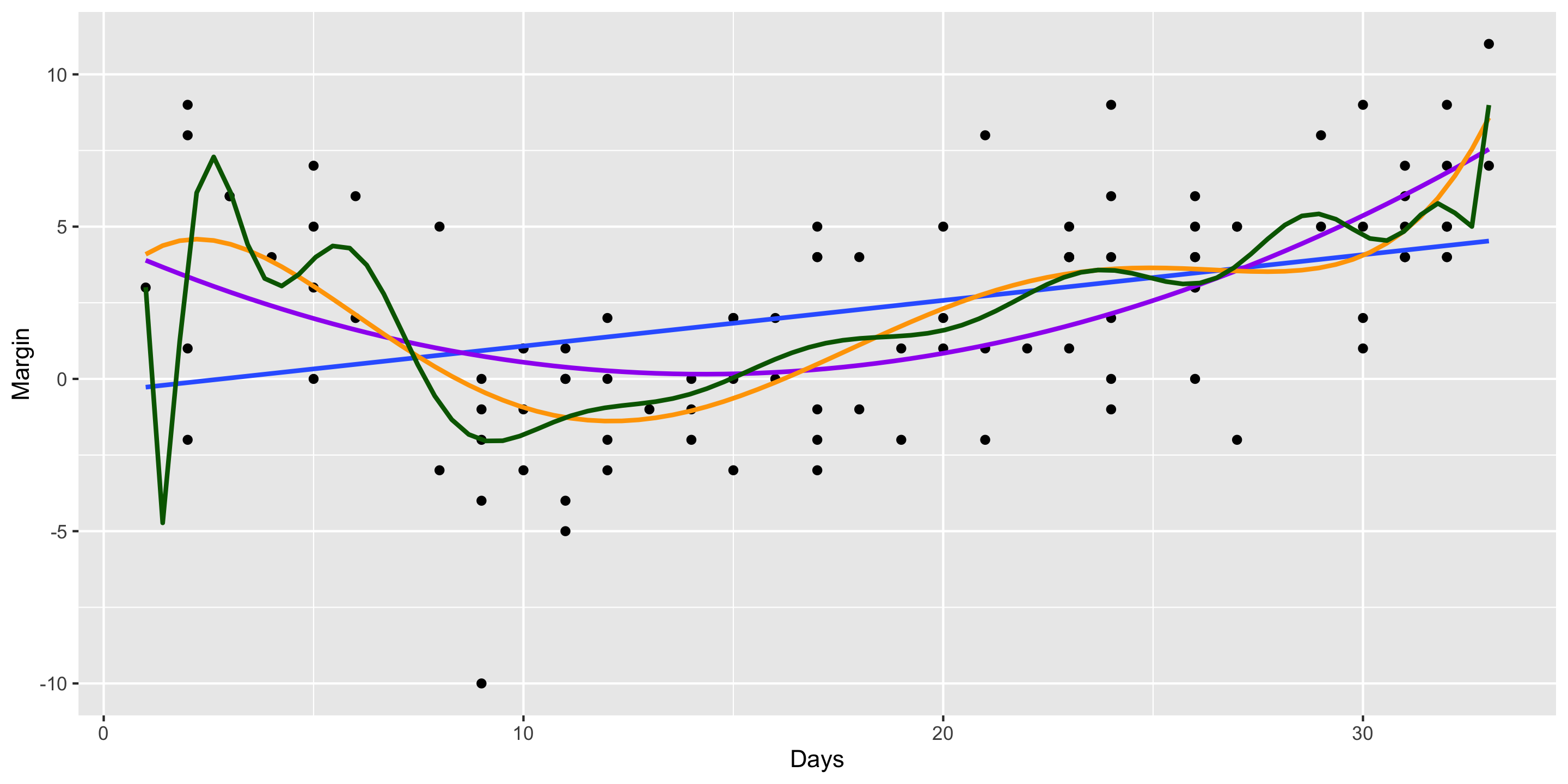
Always check your diagnostic plots to ensure the model you choose is properly specified!
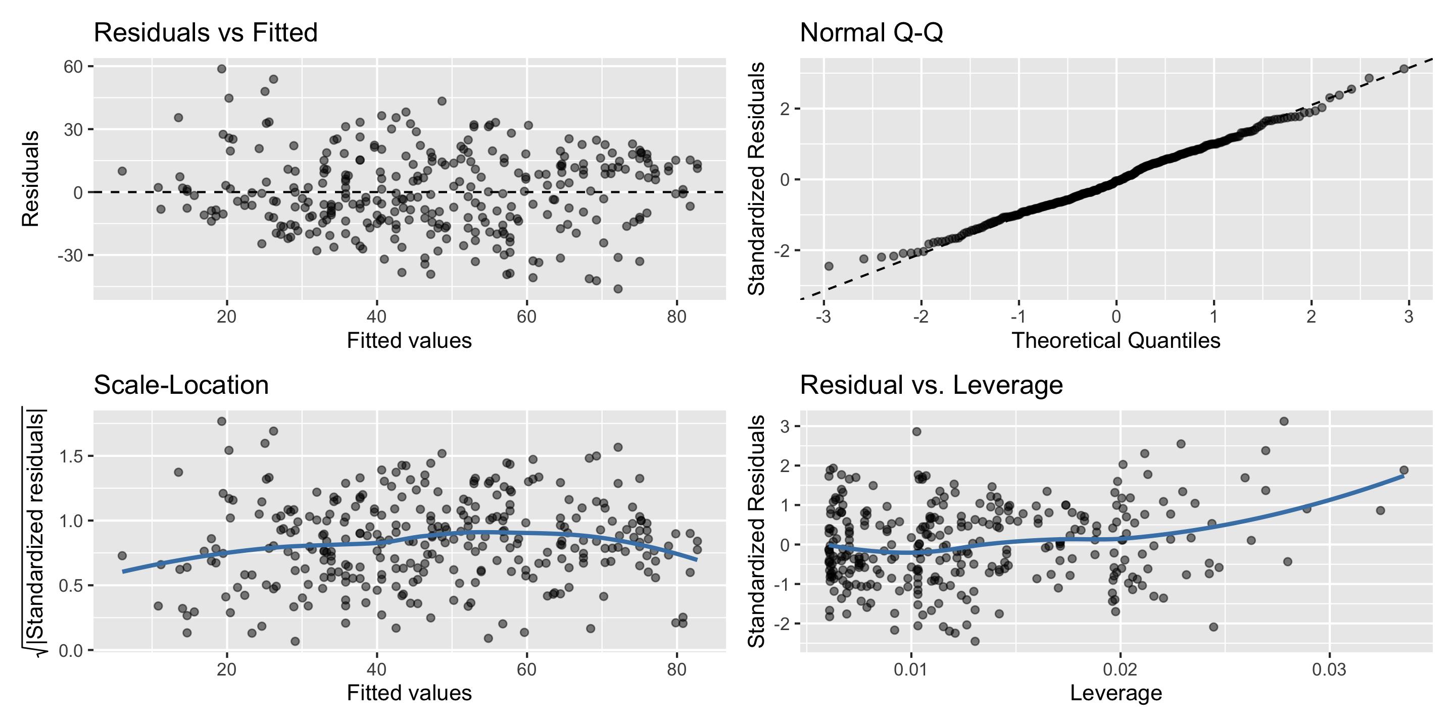
Model Building Guidance: Diagnostic Plots
Always check your diagnostic plots to ensure the model you choose is properly specified!
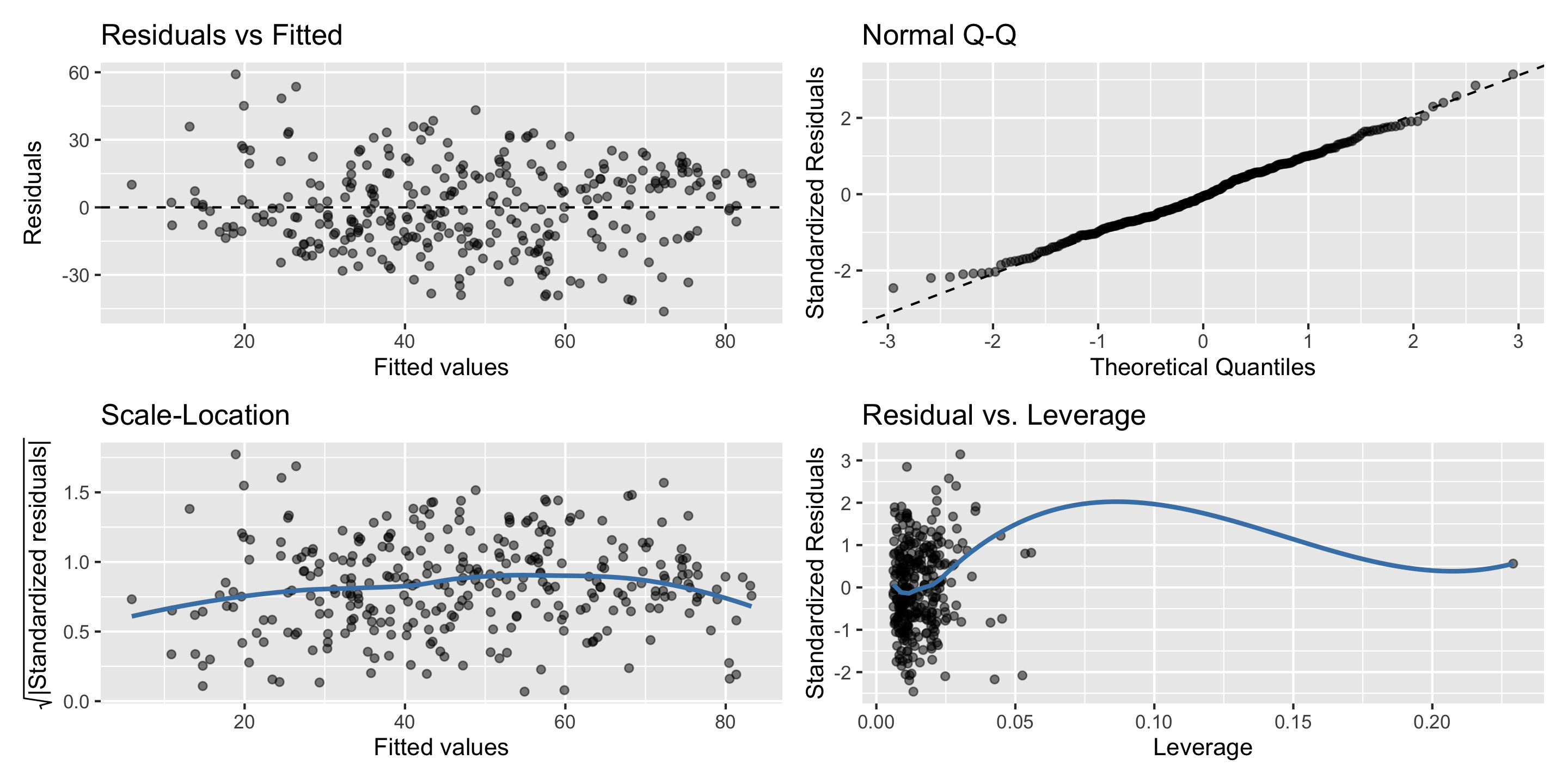
Model Building Guidance: Diagnostic Plots
Always check your diagnostic plots to ensure the model you choose is properly specified!
Model Building Guidance
We often have several potential explanatory variables. How do we determine which to include in the model and in what form?
Guiding Principle: Use your modeling motivation to determine how much you weigh interpretability versus prediction accuracy when choosing the model.