

Quantifying Uncertainty
Grayson White
Math 141
Week 6 | Fall 2025
Algorithmic Bias
Algorithmic bias: when the model systematically creates unfair outcomes, such as privileging one group over another.
Example: COMPAS model used throughout the country to predict recidivism
- Differences in predictions across race and gender
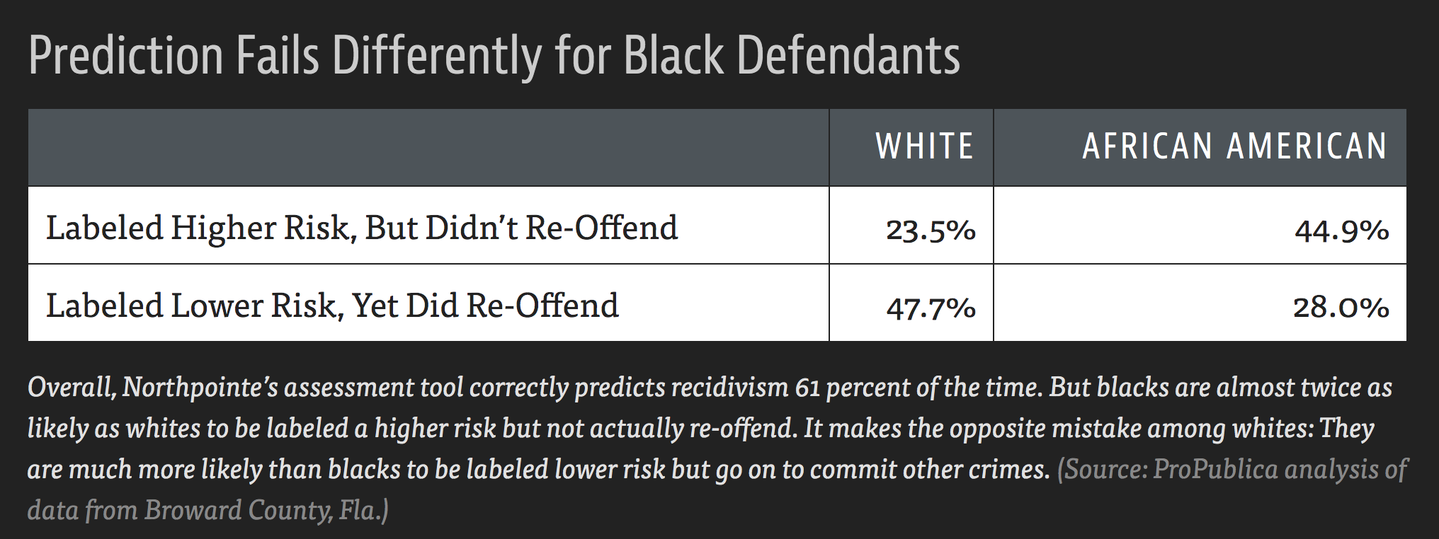
- Cynthia Rudin and collaborators wrote The Age of Secrecy and Unfairness in Recidivism Prediction
- Argue for the need for transparency in models that make such important decisions.
The ❤️ of statistical inference is quantifying uncertainty
Quantifying Our Uncertainty
R has been giving us uncertainty estimates:
library(pdxTrees)
kenilworth <- get_pdxTrees_parks() %>%
  filter(Park %in% c("Kenilworth Park")) %>%
  drop_na(Functional_Type, Native)

ggplot(kenilworth, aes(x = Tree_Height,
                       y = DBH, color = Native)) +
  geom_point() +
  stat_smooth(method = "lm", se = TRUE) +
  scale_color_manual(values = c("plum3", "goldenrod")) +
theme(legend.position = "bottom") 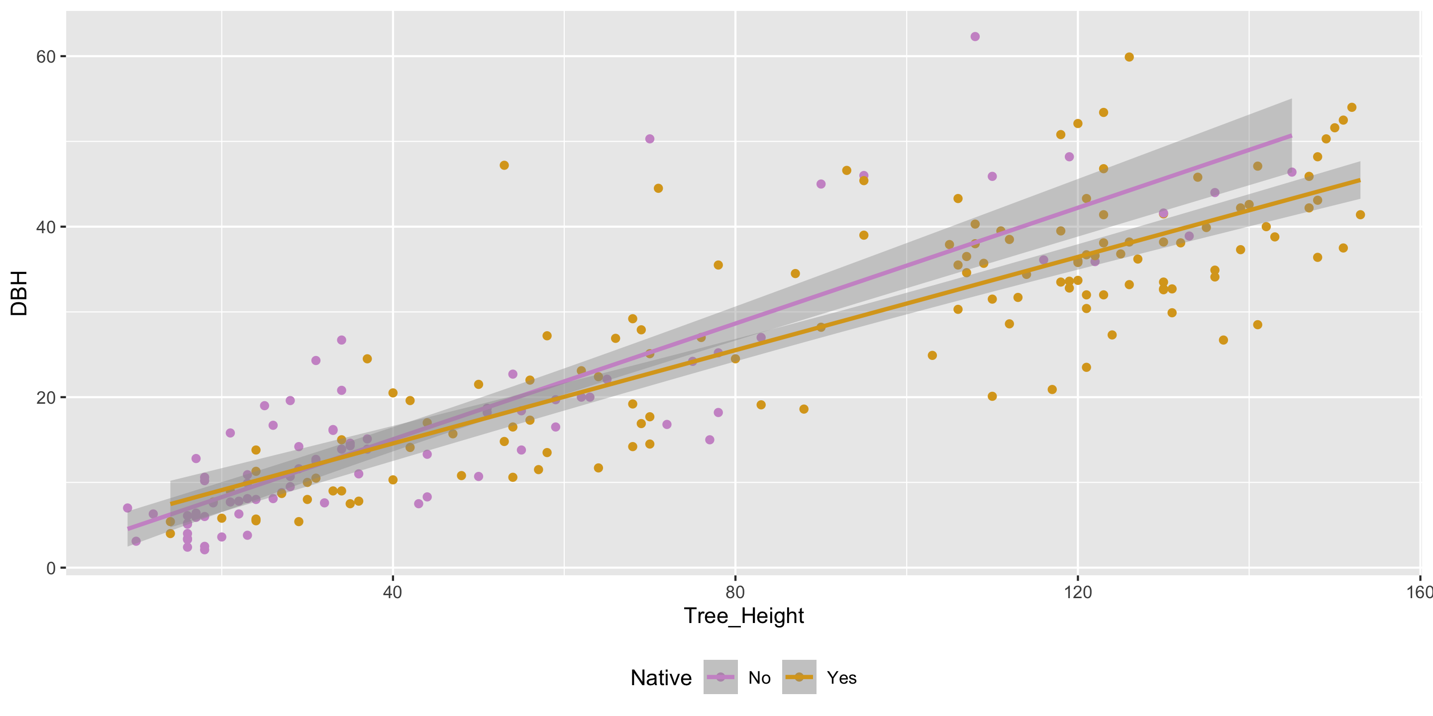
Quantifying Our Uncertainty
Uncertainty estimates are constantly reported in news and journal articles:
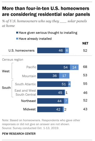
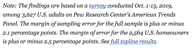
Quantifying Our Uncertainty
Uncertainty estimates are constantly reported in news and journal articles:

Statistical Inference
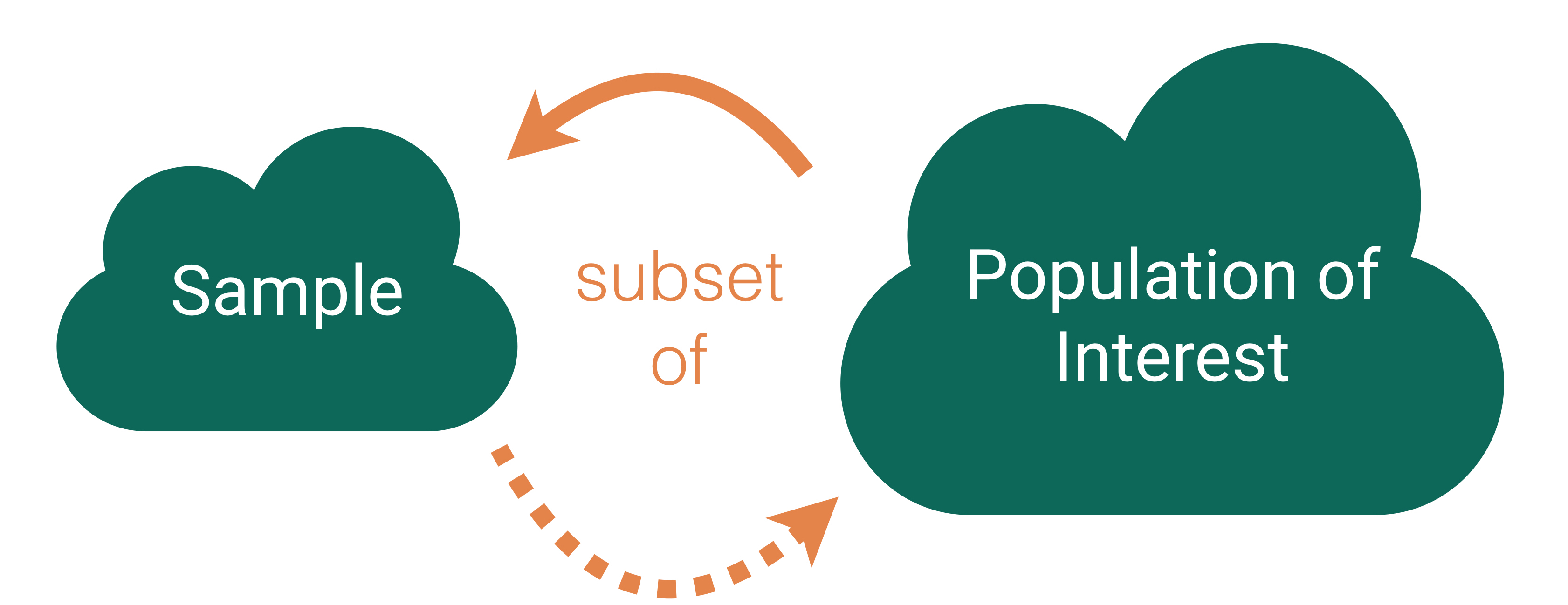
Goal: Draw conclusions about the population based on the sample.
Plato’s allegory of the cave

Sampling Distribution of a Statistic
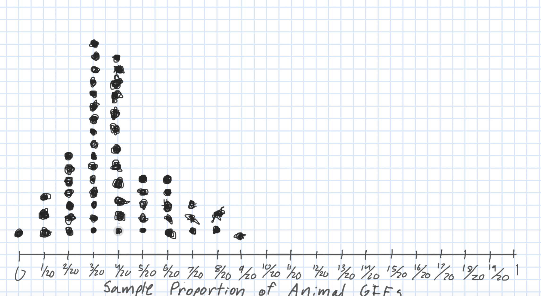
Center? Shape?
Spread?
- Standard error = standard deviation of the statistic
What happens to the center/spread/shape as we increase the sample size?
What happens to the center/spread/shape if the true parameter changes?