Quantifying Uncertainty II

Grayson White

Math 141
Week 7 | Fall 2025

Announcements

• Midterm exam available today!
  • Finish take-home by Weds 10am (2.5hr exam)
  • Make sure you’ve signed up for an oral exam time!
• Discussion of midterm logistics (cloning repo, Gradescope process, rendering, office hours)

Goals for Today

• Continue our discussion of quantifying uncertainty
  • Key ideas:
    • sampling variability, sampling distributions, populations, samples, parameters, statistics.

• Construct sampling distributions in R

Statistical Inference

The ❤️ of statistical inference is quantifying uncertainty

library(tidyverse)
ce <- read_csv("data/fmli.csv")
summarize(ce, meanFINCBTAX = mean(FINCBTAX))

# A tibble: 1 × 1
  meanFINCBTAX
         <dbl>
1       62480.

The ❤️ of statistical inference is quantifying uncertainty

library(tidyverse)
ce <- read_csv("data/fmli.csv")
summarize(ce, meanFINCBTAX = mean(FINCBTAX))

# A tibble: 1 × 1
  meanFINCBTAX
         <dbl>
1       62480.

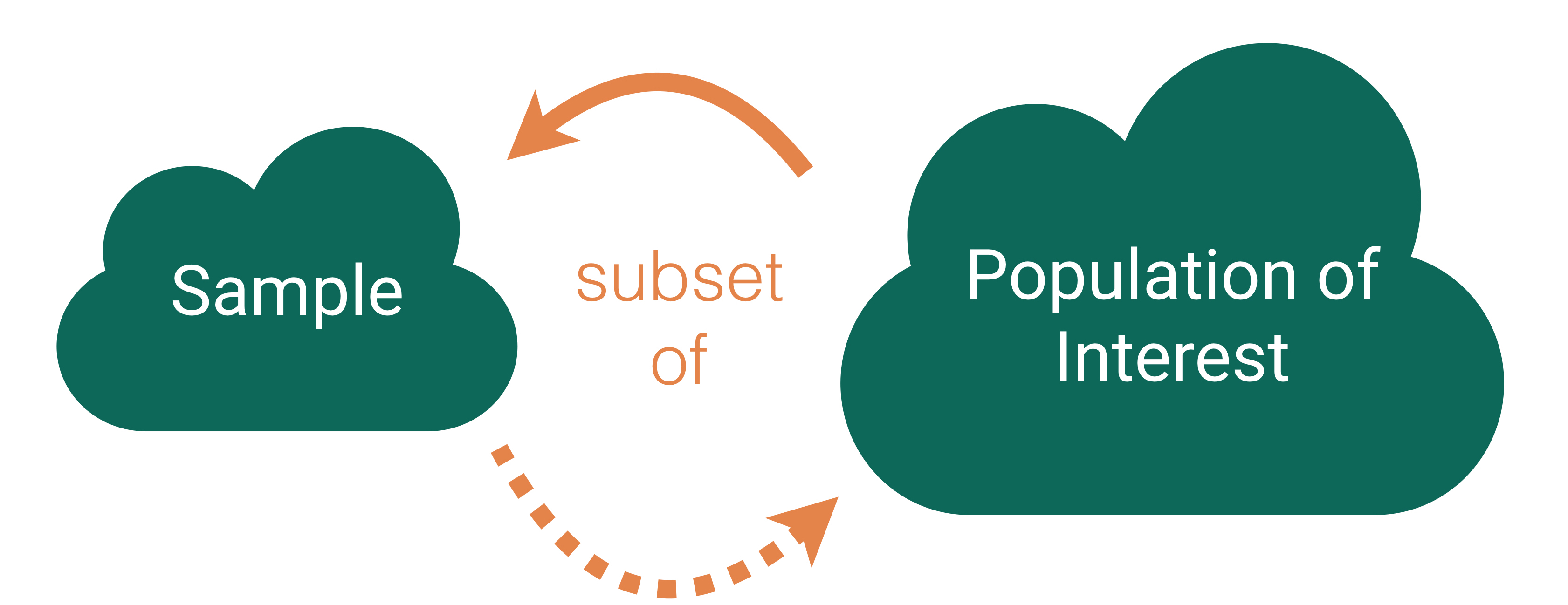
Like with regression, need to distinguish between the population and the sample

• Parameters:
  • Based on the population
  • Unknown then if don’t have data on the whole population
  • EX: \(\beta_o\) and \(\beta_1\)
  • EX: \(\mu\) = population mean

• Statistics:
  • Based on the sample data
  • Known
  • Usually estimate a population parameter
  • EX: \(\hat{\beta}_o\) and \(\hat{\beta}_1\)
  • EX: \(\bar{x}\) = sample mean

Statistical Inference

Goal: Draw conclusions about the population based on the sample.

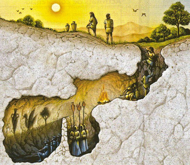
Plato’s allegory of the cave

Statistical Inference

Goal: Draw conclusions about the population based on the sample.

Main Flavors

• Estimating numerical quantities (parameters).

• Testing conjectures.

Estimation

Goal: Estimate a (population) parameter.

Best guess?

• The corresponding (sample) statistic

Key Question: How accurate is the statistic as an estimate of the parameter?

Helpful Sub-Question: If we take many samples, how much would the statistic vary from sample to sample?

Need two new concepts:

• The sampling variability of a statistic

• The sampling distribution of a statistic

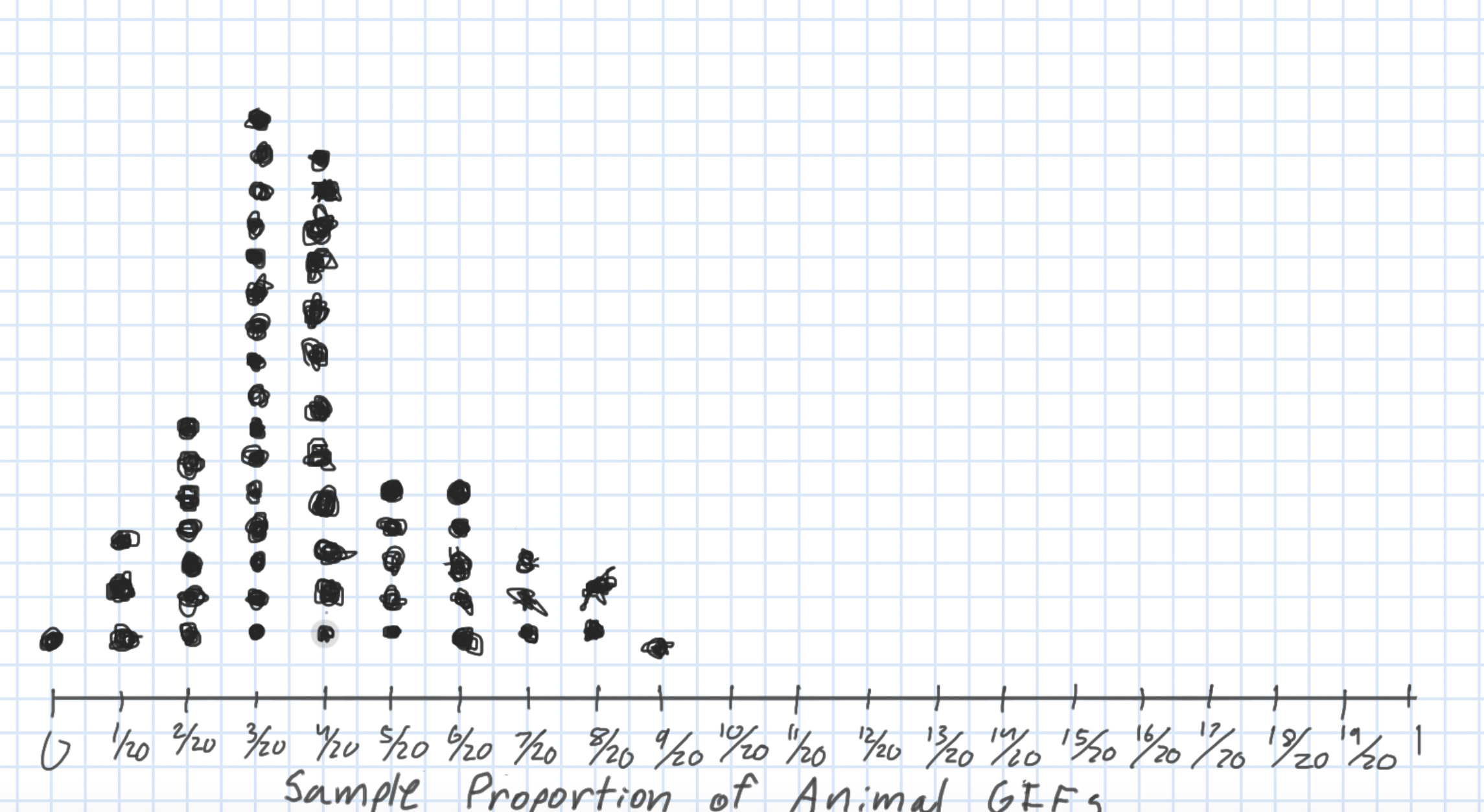
Sampling Distribution of a Statistic

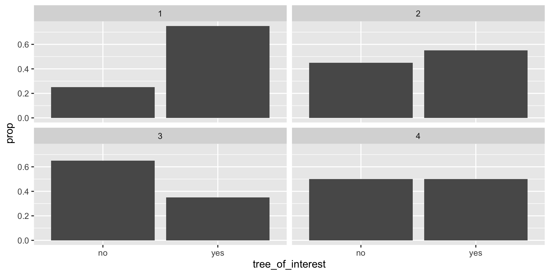
Steps to Construct an (Approximate) Sampling Distribution:

1. Decide on a sample size, \(n\).

2. Randomly select a sample of size \(n\) from the population.

3. Compute the sample statistic.

4. Put the sample back in.

5. Repeat Steps 2 - 4 many (1000+) times.

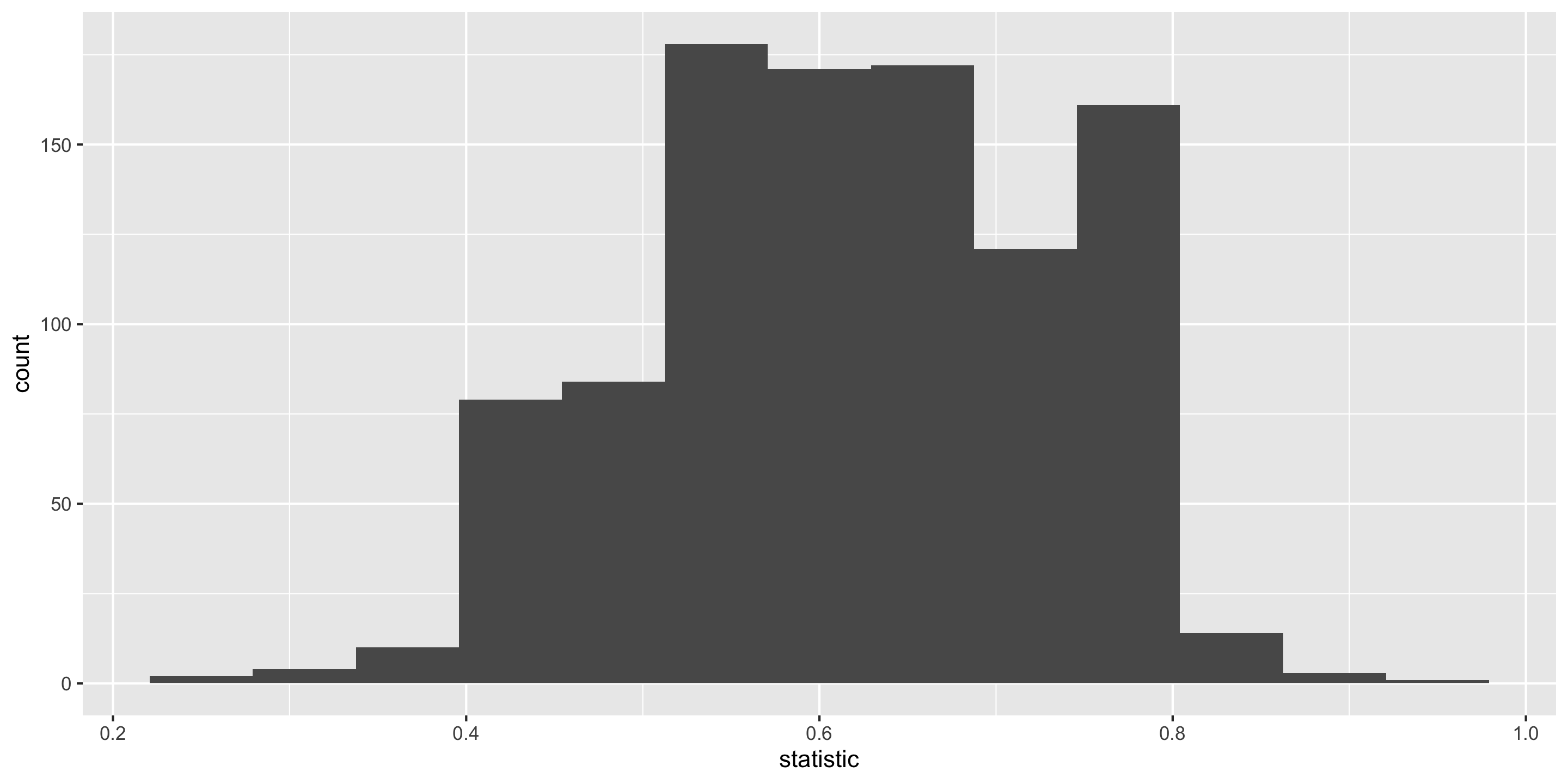
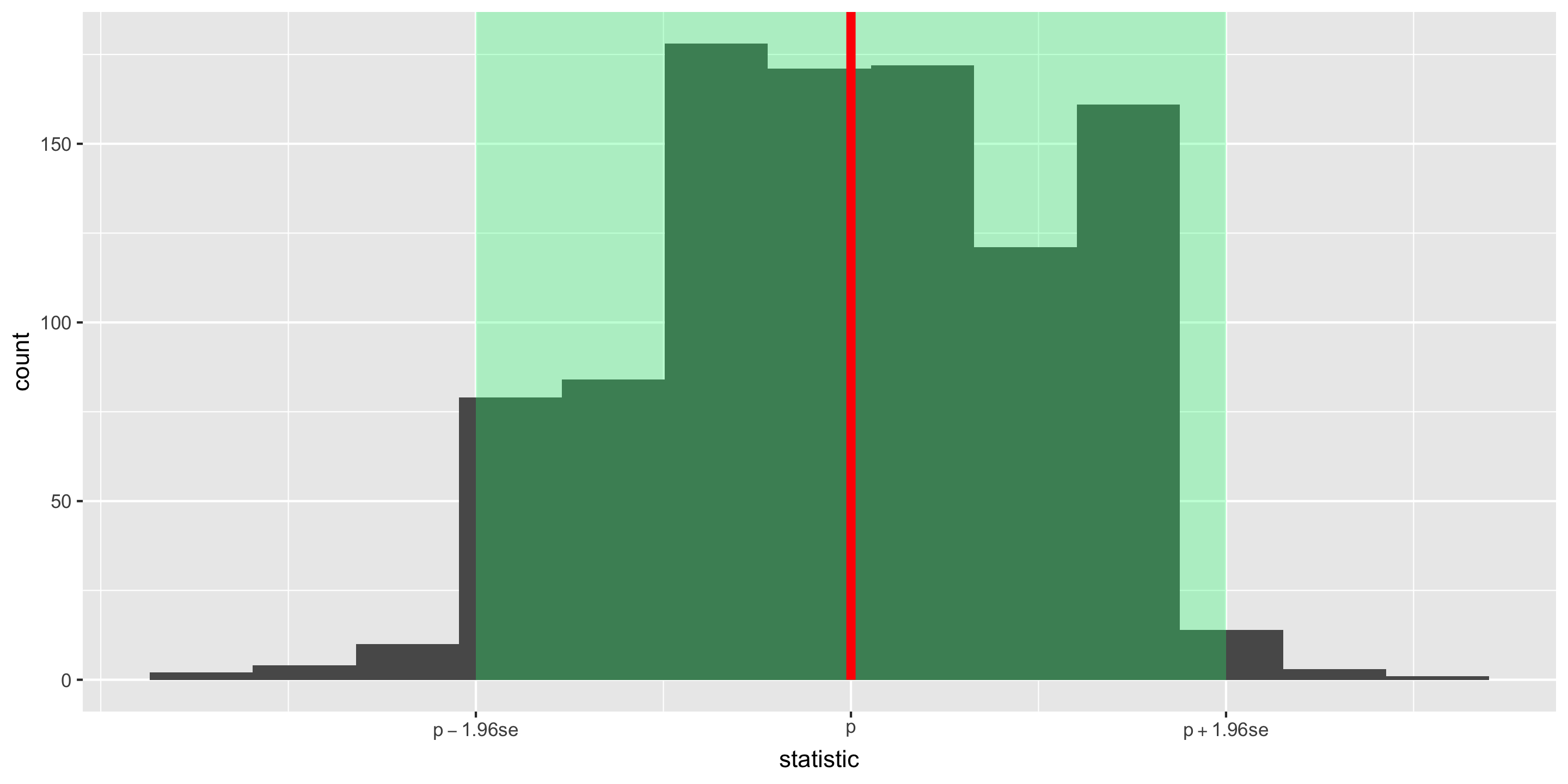
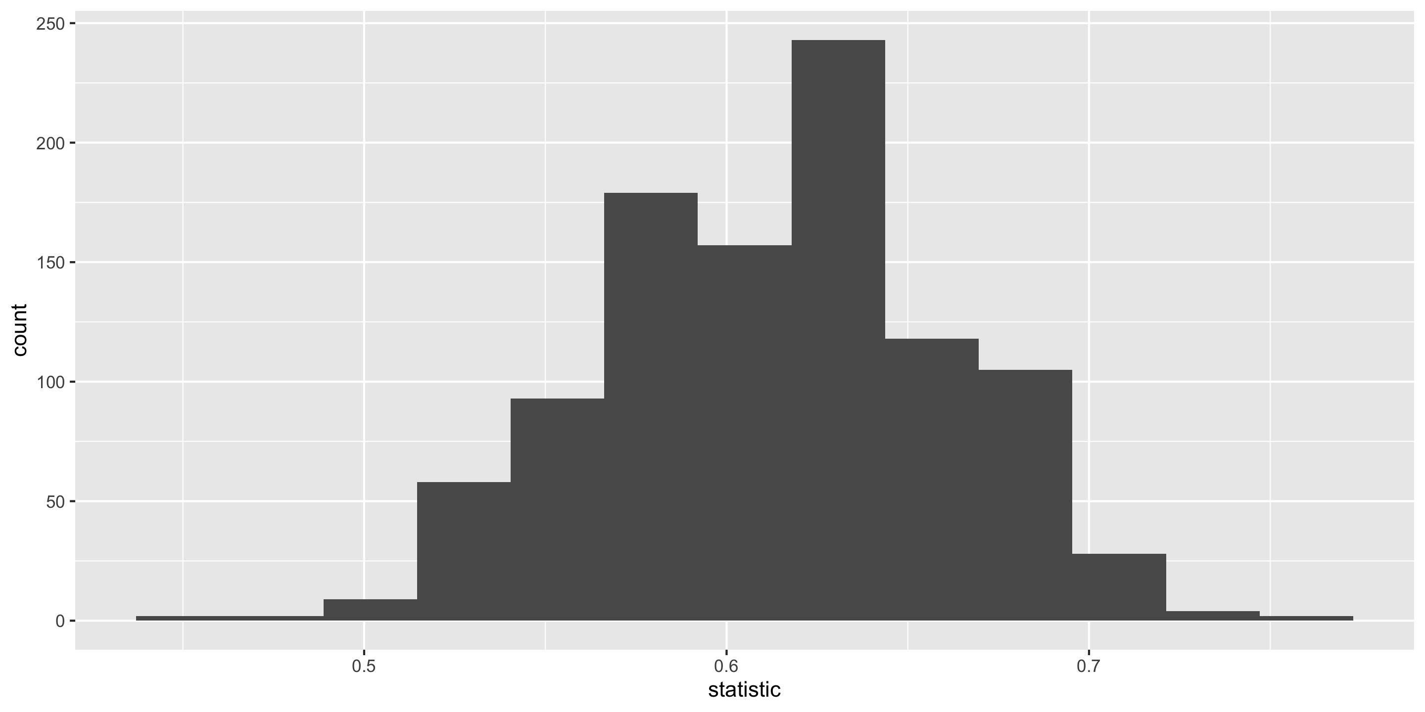
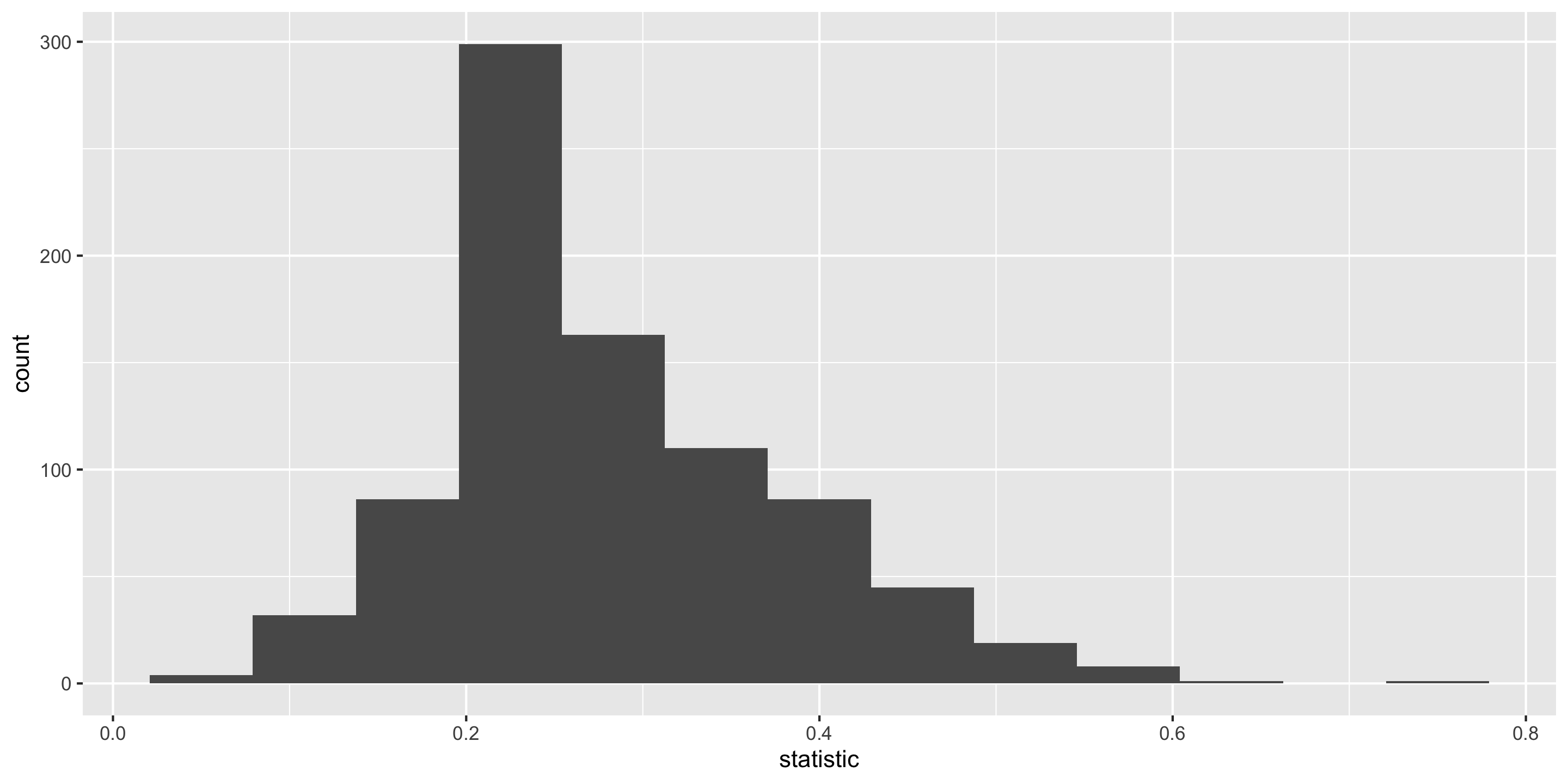
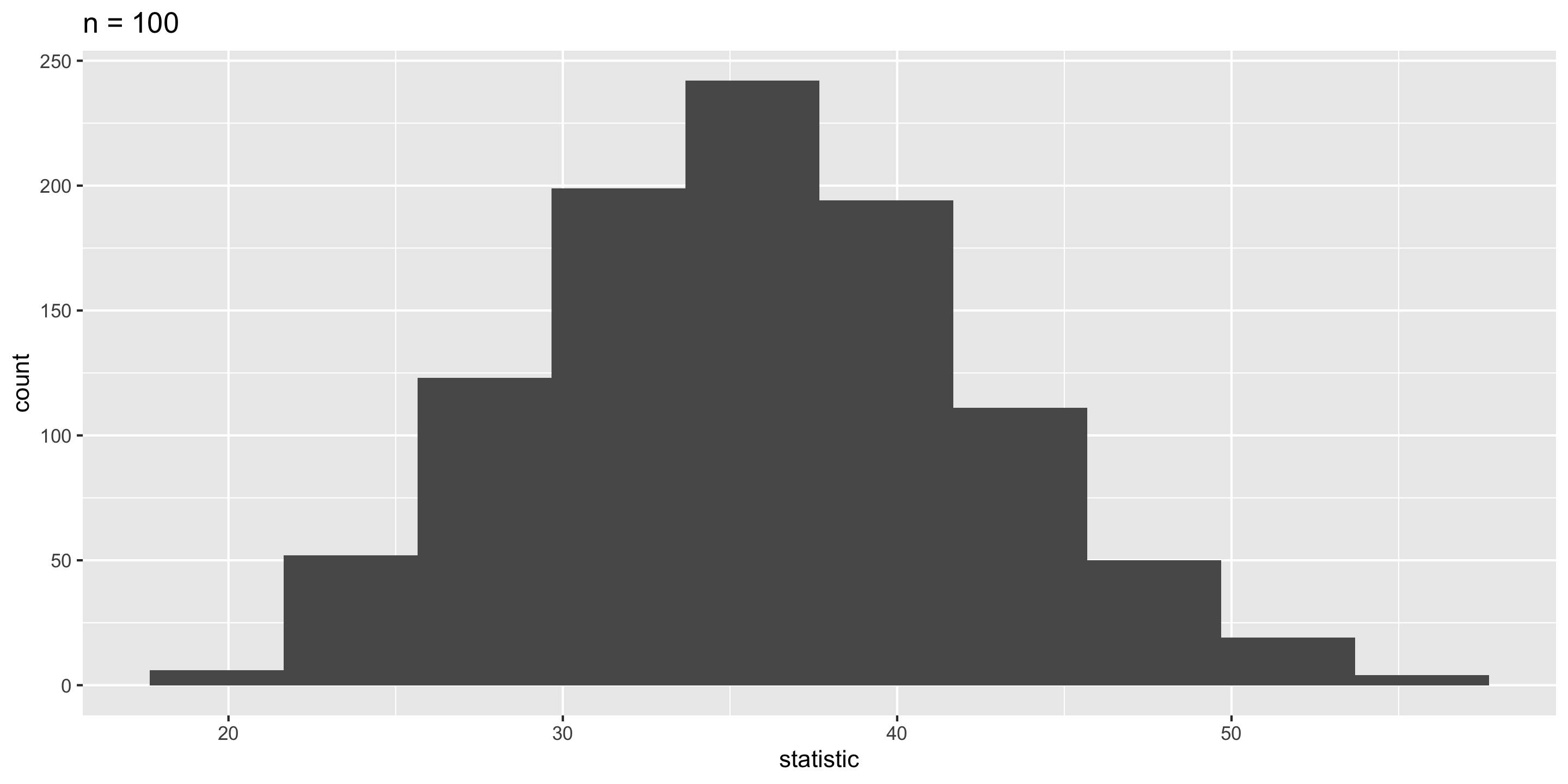
Sampling Distribution of a Statistic

• Center? Shape?

• Spread?

  • Standard error = standard deviation of the statistic

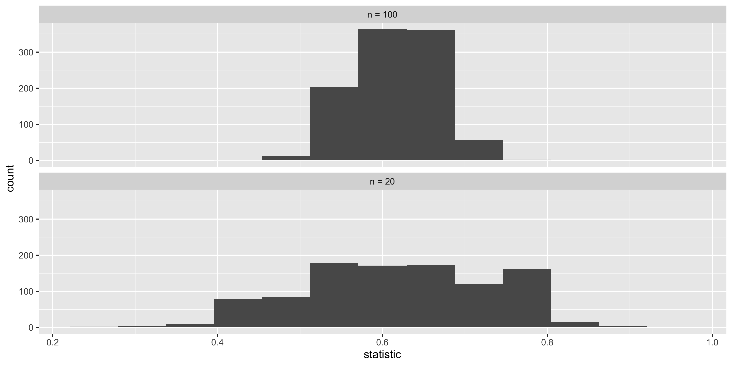
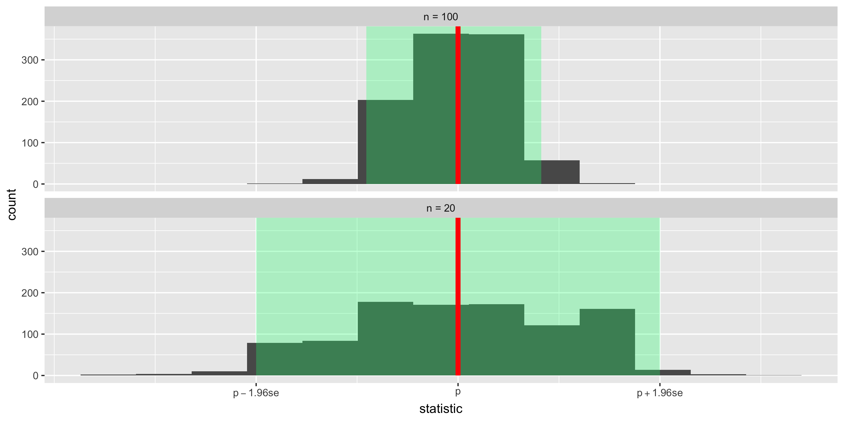
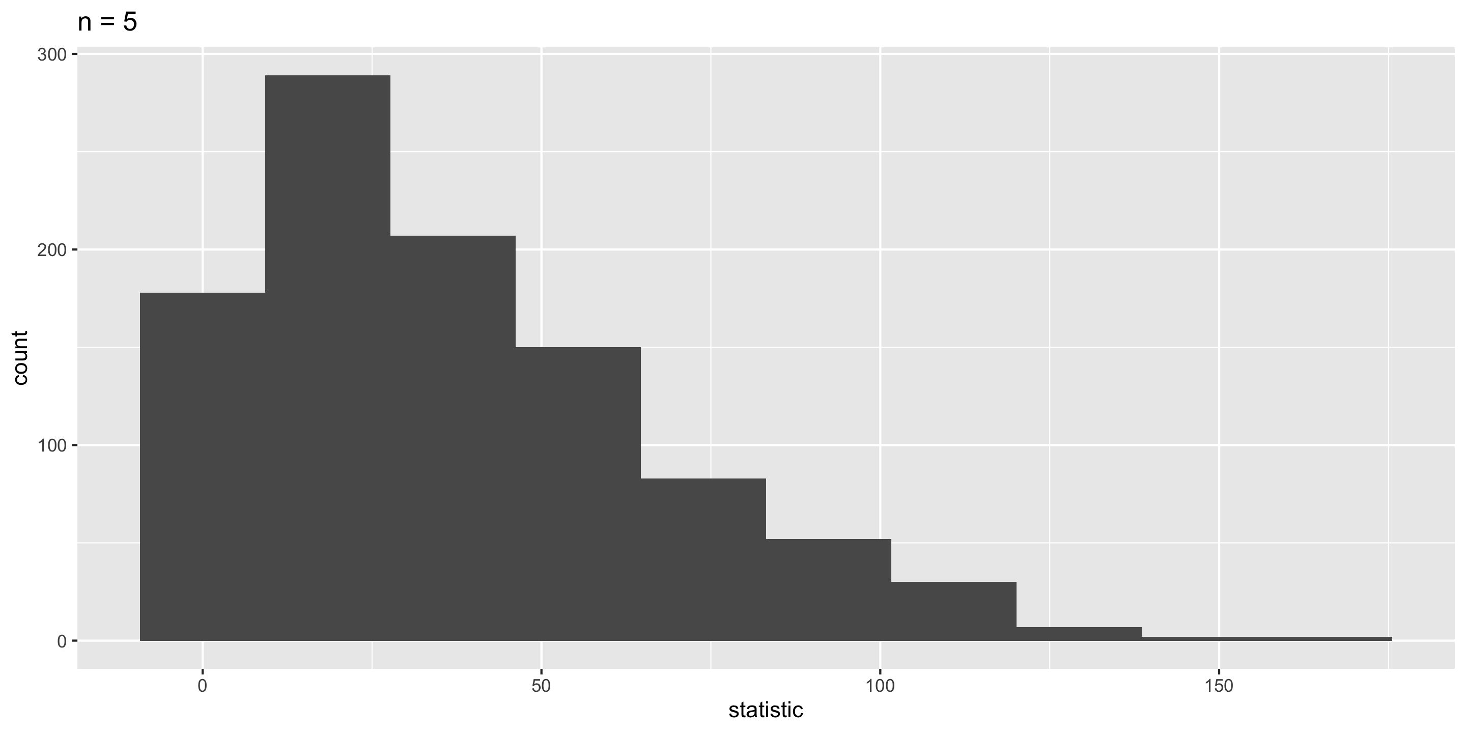
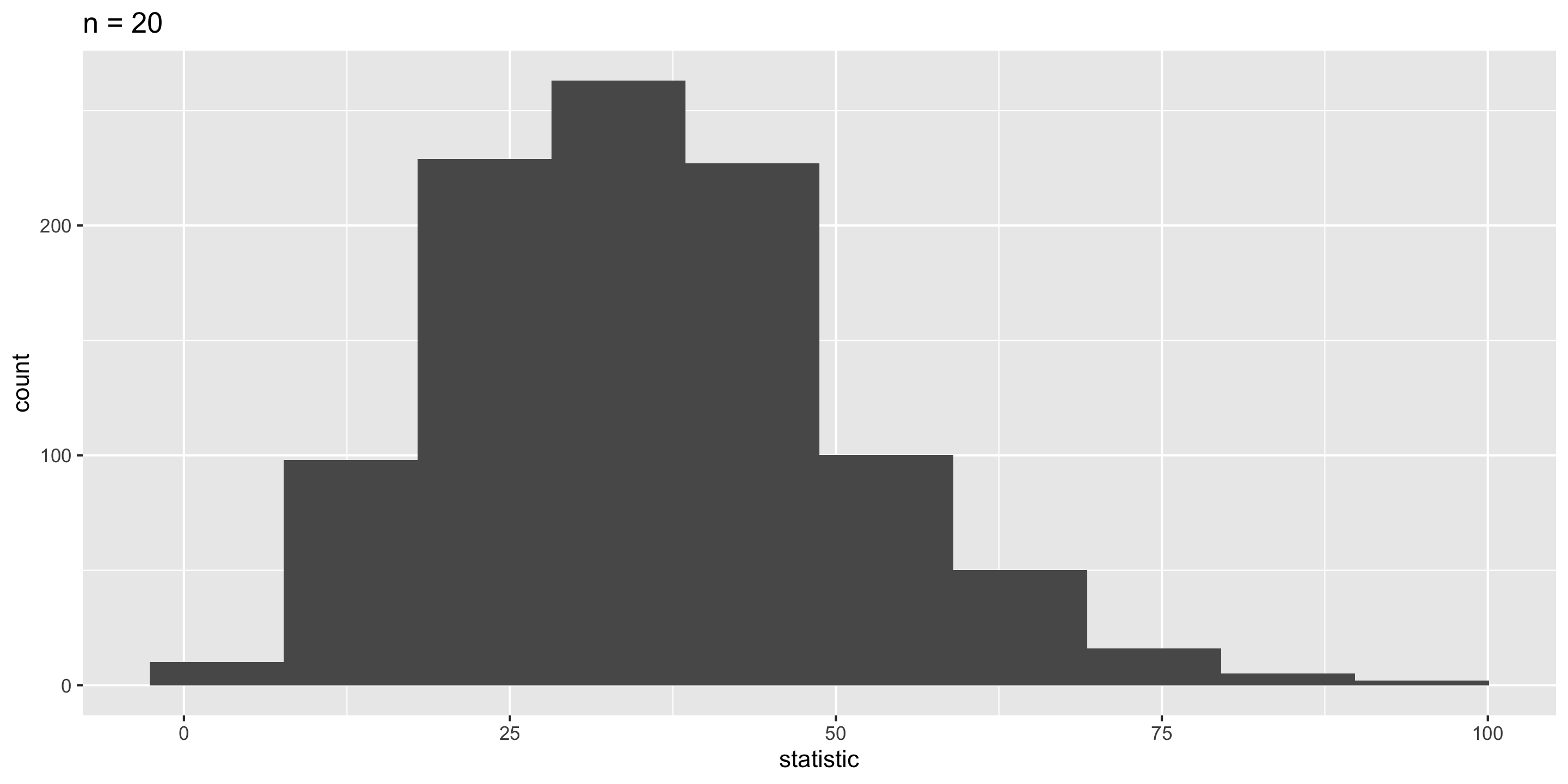
• What happens to the center/spread/shape as we increase the sample size?

• What happens to the center/spread/shape if the true parameter changes?

Let’s Construct Some Sampling Distributions using R!

Important Notes

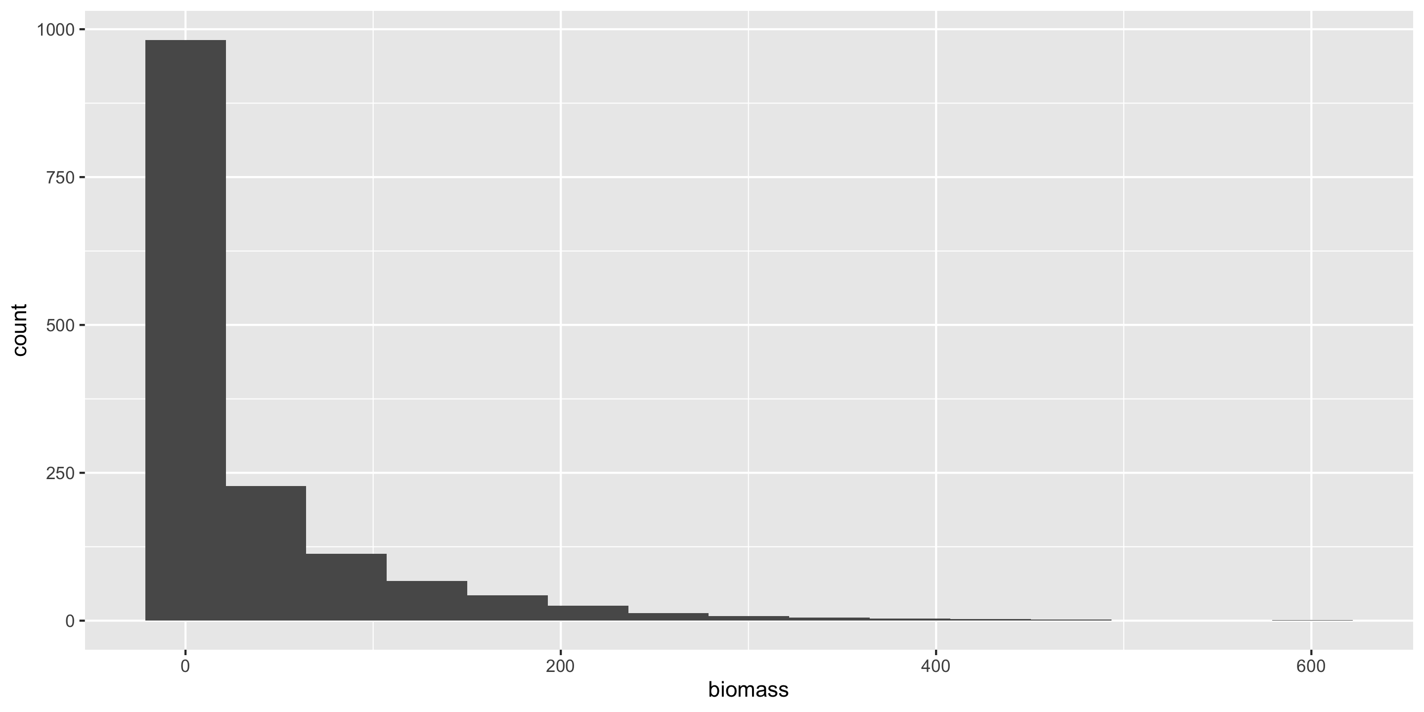
• To construct a sampling distribution for a statistic, we need access to the entire population so that we can take repeated samples from the population.

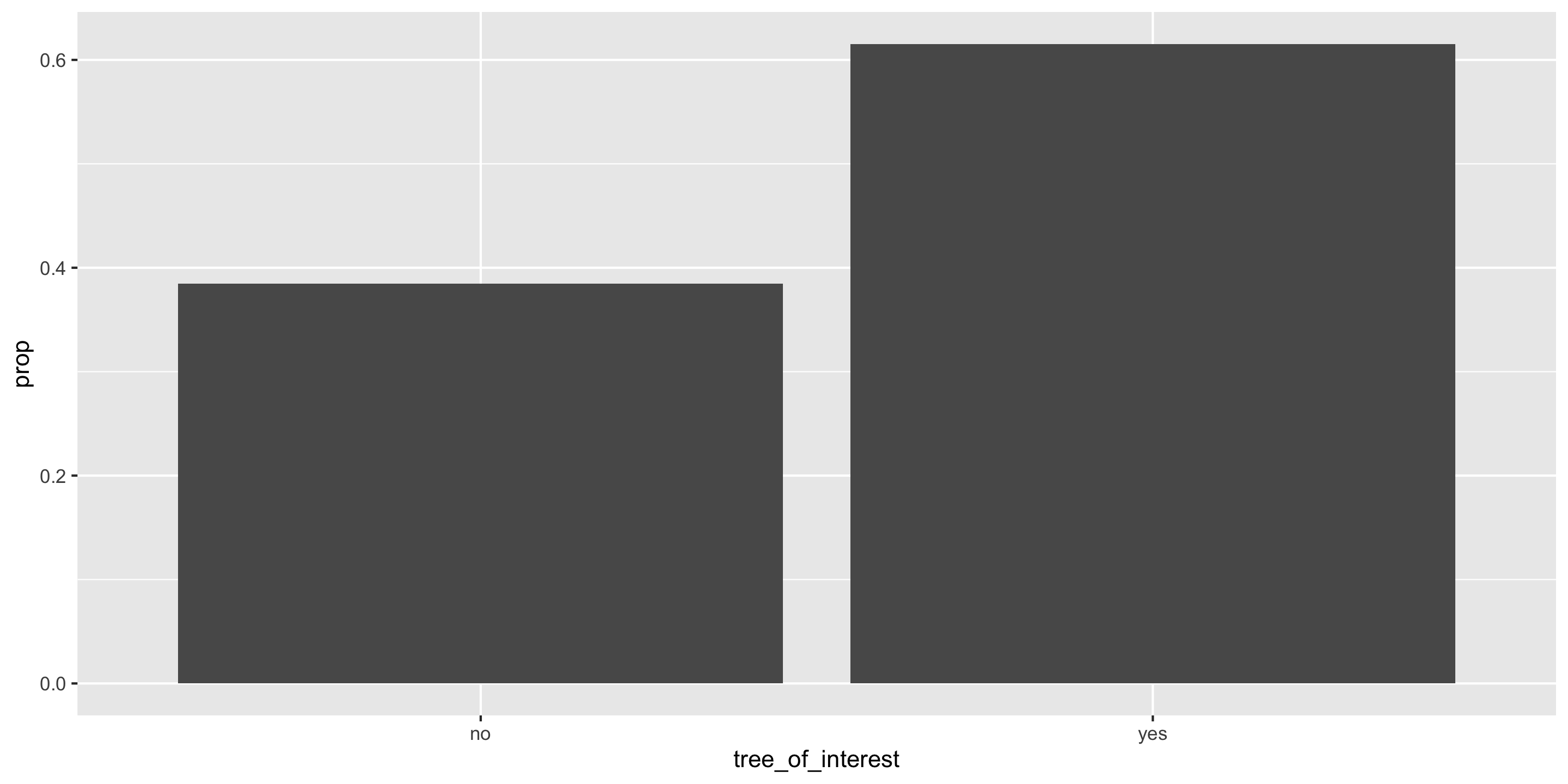
  • Population = Mt Tabor trees

• But if we have access to the entire population, then we know the value of the population parameter.

  • Can compute the exact proportion of maple trees in our population.

• The sampling distribution is needed in the exact scenario where we can’t compute it: the scenario where we only have a single sample.

• We will learn how to estimate the sampling distribution soon.

• Today, we have the entire population and are constructing sampling distributions anyway to study their properties!

New R Package: infer

library(infer)

New R Package: infer

library(infer)

• Will use infer to conduct statistical inference.

Our Population Parameter

Create data frame of Mt Tabor trees:

library(tidyverse)
library(pdxTrees)
tabor <- get_pdxTrees_parks(park = "Mt Tabor Park")

Add variable of interest:

tabor <- tabor %>%
  mutate(tree_of_interest = case_when(
    Genus == "Pseudotsuga" ~ "yes",
    Genus != "Pseudotsuga" ~ "no"
  ))
count(tabor, tree_of_interest)

# A tibble: 2 × 2
  tree_of_interest     n
  <chr>            <int>
1 no                 435
2 yes                696

Population Parameter

# Population distribution
ggplot(data = tabor, 
       mapping = aes(x = tree_of_interest)) +
  geom_bar(aes(y = after_stat(prop), group = 1)) 

# True population parameter
tabor %>%
  summarize(parameter = mean(tree_of_interest == "yes"))

# A tibble: 1 × 1
  parameter
      <dbl>
1     0.615

Random Samples

Let’s look at 4 random samples.

# Draw random samples
samples <- tabor %>% 
  rep_sample_n(size = 20, reps = 4)
  
# Graph the samples
ggplot(data = samples, 
       mapping = aes(x = tree_of_interest)) +
  geom_bar(aes(y = after_stat(prop), group = 1)) +
  facet_wrap(~replicate)

Constructing the Sampling Distribution

Now, let’s take 1000 random samples.

# Construct the sampling distribution
samp_dist <- tabor %>% 
  rep_sample_n(size = 20, reps = 1000) %>%
  group_by(replicate) %>%
  summarize(
    statistic = mean(tree_of_interest == "yes")
    )

# Graph the sampling distribution
ggplot(data = samp_dist, 
       mapping = aes(x = statistic)) +
  geom_histogram(bins = 13)

• Shape?

• Center?

• Spread?

Properties of the Sampling Distribution

summarize(samp_dist, estimate = mean(statistic))

# A tibble: 1 × 1
  estimate
     <dbl>
1    0.618

summarize(samp_dist, standard_error = sd(statistic))

# A tibble: 1 × 1
  standard_error
           <dbl>
1          0.108

The standard deviation of a sample statistic is called the standard error.

Properties of the Sampling Distribution

summarize(samp_dist, estimate = mean(statistic))

# A tibble: 1 × 1
  estimate
     <dbl>
1    0.618

summarize(samp_dist, standard_error = sd(statistic))

# A tibble: 1 × 1
  standard_error
           <dbl>
1          0.108

For approximately bell-shaped distributions, about 95% of observations fall within 1.96 standard deviations of the population’s mean \(p\).

Huge Implication:

• The sampling distribution for the mean, \(\hat p\) is approximately bell-shaped

• … and is centered at the population mean, \(p\).

• So 95% of all sample statistics, \(\hat p\) fall within 1.96 standard errors of \(p\)!

What happens to the sampling distribution if we change the sample size from 20 to 100?

# Construct the sampling distribution
samp_dist_100 <- tabor %>% 
  rep_sample_n(size = 100, reps = 1000) %>%
  group_by(replicate) %>%
  summarize(
    statistic = mean(tree_of_interest == "yes")
    )

# Graph the sampling distribution
ggplot(data = samp_dist_100, 
       mapping = aes(x = statistic)) +
  geom_histogram(bins = 13)

summarize(samp_dist_100, mean(statistic), 
          sd(statistic))

# A tibble: 1 × 2
  `mean(statistic)` `sd(statistic)`
              <dbl>           <dbl>
1             0.613          0.0469

Changing sample size

• As the size of our sample increases, the variability of the sampling distribution decreases.

• This makes sense: more data –> more precise estimates

Changing sample size

• Both sampling distributions are still centered at \(p\), but

• We can see that 95% of samples lie within different ranges for different \(n\)

• As \(n\) increases, sampling variability (i.e. the standard error of the sampling distribution) decreases

What if we change the true parameter value?

# Construct the sampling distribution
samp_dist <- tabor %>%
  rep_sample_n(size = 20, reps = 1000) %>%
  group_by(replicate) %>%
  summarize(
    statistic = mean(Functional_Type == "BD")
    )

# Graph the sampling distribution
ggplot(data = samp_dist,
       mapping = aes(x = statistic)) +
    geom_histogram(bins = 13)

summarize(samp_dist, mean(statistic, na.rm = TRUE),
          sd(statistic, na.rm = TRUE))

# A tibble: 1 × 2
  `mean(statistic, na.rm = TRUE)` `sd(statistic, na.rm = TRUE)`
                            <dbl>                         <dbl>
1                           0.284                         0.101

A Word of Warning: The Shape of the Sampling Distribution

Sometimes, you need a large enough sample for your sampling distribution to look bell-shaped.

Example: forest biomass in Oregon

oregon_biomass %>%
  ggplot(aes(x = biomass)) + 
  geom_histogram(bins = 15)

A Word of Warning: The Shape of the Sampling Distribution

Sometimes, you need a large enough sample for your sampling distribution to look bell-shaped.

Example: forest biomass in Oregon

oregon_5 <- oregon_biomass %>%
  rep_sample_n(size = 5, reps = 1000)

oregon_5 %>%
  group_by(replicate) %>%
  summarize(statistic = mean(biomass)) %>%
  ggplot(aes(x = statistic)) +
  geom_histogram(bins = 10) +
  labs(title = "n = 5")

A Word of Warning: The Shape of the Sampling Distribution

Sometimes, you need a large enough sample for your sampling distribution to look bell-shaped.

Example: forest biomass in Oregon

oregon_20 <- oregon_biomass %>%
  rep_sample_n(size = 20, reps = 1000)

oregon_20 %>%
  group_by(replicate) %>%
  summarize(statistic = mean(biomass)) %>%
  ggplot(aes(x = statistic)) +
  geom_histogram(bins = 10) + 
  labs(title = "n = 20")

A Word of Warning: The Shape of the Sampling Distribution

Sometimes, you need a large enough sample for your sampling distribution to look bell-shaped.

Example: forest biomass in Oregon

oregon_100 <- oregon_biomass %>%
  rep_sample_n(size = 100, reps = 1000)

oregon_100 %>%
  group_by(replicate) %>%
  summarize(statistic = mean(biomass)) %>%
  ggplot(aes(x = statistic)) +
  geom_histogram(bins = 10) + 
  labs(title = "n = 100")

On Lab 6:

Will investigate what happens when we change the parameter of interest to a mean or a correlation coefficient!

Key Features of a Sampling Distribution

What did we learn about sampling distributions?

• Centered around the true population parameter.

• As the sample size increases, the standard error (SE) of the statistic decreases.

• As the sample size increases, the shape of the sampling distribution becomes more bell-shaped and symmetric.

Question:

How do sampling distributions help us quantify uncertainty?

Question:

If I am estimating a parameter in a real example, why won’t I be able to construct the sampling distribution?

Cliffhanger:

How can I quantify uncertainty in a sample statistic when I only have access to one sample??