Grab 30 notecards! It is okay if they already have markings on them. And, please return the notecards to the same spot after class.


The Bootstrap


Grayson White

Math 141
Week 7 | Fall 2025

Announcements

  • Last class before fall break!

  • Instead of class on Thursday and Friday, we’ll be having oral exams.

  • No office hours for the rest of the week (starting today).

Goals for Today

  • Recall ideas about the sampling distribution
  • Learn how to approximate the sampling distribution via bootstrapping
  • Learn about confidence intervals

Statistical Inference

Goal: Draw conclusions about the population based on the sample.

Main Flavors

  • Estimating numerical quantities (parameters).

  • Testing conjectures.

Sampling Distribution of a Statistic

Steps to Construct an (Approximate) Sampling Distribution:

  1. Decide on a sample size, \(n\).

  2. Randomly select a sample of size \(n\) from the population.

  3. Compute the sample statistic.

  4. Put the sample back in.

  5. Repeat Steps 2 - 4 many (1000+) times.

Sampling Distribution of a Statistic

  • What are some of the key features of a sampling distribution?

  • How do sampling distributions help us quantify uncertainty?

  • If I am estimating a parameter in a real example, why won’t I be able to construct the sampling distribution?

Estimation

Goal: Estimate the value of a population parameter using data from the sample.

  • Question: How do I know which population parameter I am interesting in estimating?

  • Answer: Likely depends on the research question and structure of your data!

  • Point Estimate: The corresponding statistic

    • Single best guess for the parameter

Remember: Plato’s Cave.

Confidence Intervals

It is time to move beyond just point estimates to interval estimates that quantify our uncertainty.

Last time, we took many (1000) samples of size 20 from the population of trees in Mt Tabor to approximate the sampling distribution

# Construct the sampling distribution
samp_dist <- tabor %>% 
  rep_sample_n(size = 20, reps = 1000) %>%
  group_by(replicate) %>%
  summarize(
    statistic = mean(tree_of_interest == "yes")
    )

# Graph the sampling distribution
ggplot(data = samp_dist, 
       mapping = aes(x = statistic)) +
  geom_histogram(bins = 33)

Confidence Intervals

It is time to move beyond just point estimates to interval estimates that quantify our uncertainty.

We saw that 95% of all samples fell within 1.96 standard errors from the center of the (approximate) sampling distribution.

Confidence Intervals

It is time to move beyond just point estimates to interval estimates that quantify our uncertainty.

This quite naturally introduces us to the idea of confidence intervals:

  • Confidence Interval: Interval of plausible values for a parameter

  • Form: \(\mbox{statistic} \pm \mbox{Margin of Error}\)

  • Question: How do we find the Margin of Error (ME)?

  • Answer: If the sampling distribution of the statistic is approximately bell-shaped and symmetric, then a statistic will be within 1.96 SEs of the parameter for 95% of the samples.

  • Form: \(\mbox{statistic} \pm 1.96\times\mbox{SE}\)

  • Called a 95% confidence interval (CI). (Will discuss the meaning of confidence soon)

Confidence Intervals

95% CI Form:

\[ \mbox{statistic} \pm 1.96\times\mbox{SE} \]

It is easy to compute a statistic for the form above (sample proportion, sample mean, …)

But… What else do we need to construct the CI?

  • Problem: To compute the SE, we need many samples from the population. We have 1 sample.

  • Solution: Approximate the sampling distribution using ONLY OUR ONE SAMPLE!

Bootstrapping

  • The term bootstrapping refers to the phrase “to pull oneself up by one’s bootstraps”

    • The phrase originated in the 19th century as reference to a ludicrous or impossible feat

    • By the mid 20th century, its meaning had changed to suggest a success by one’s own efforts, without outside help (the “American Dream” myth)

  • Its use in statistics (dating from 1979) alludes to both interpretations.

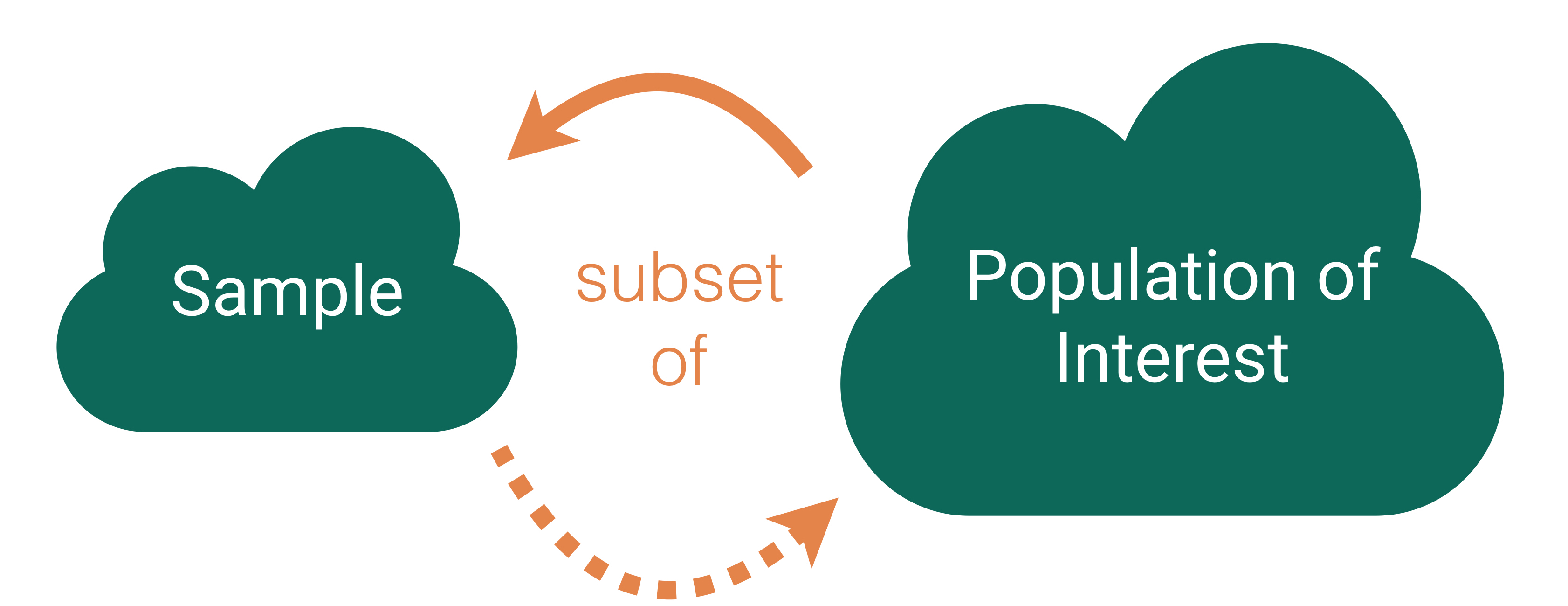
The Impossible Task:

  • How can we learn about the sampling distribution, if we only have 1 sample?

The “Ludicrous” Solution obtained without outside help:

  • Draw repeated samples from the original sample at hand; compute the statistic of interest for each; plot the resulting distribution

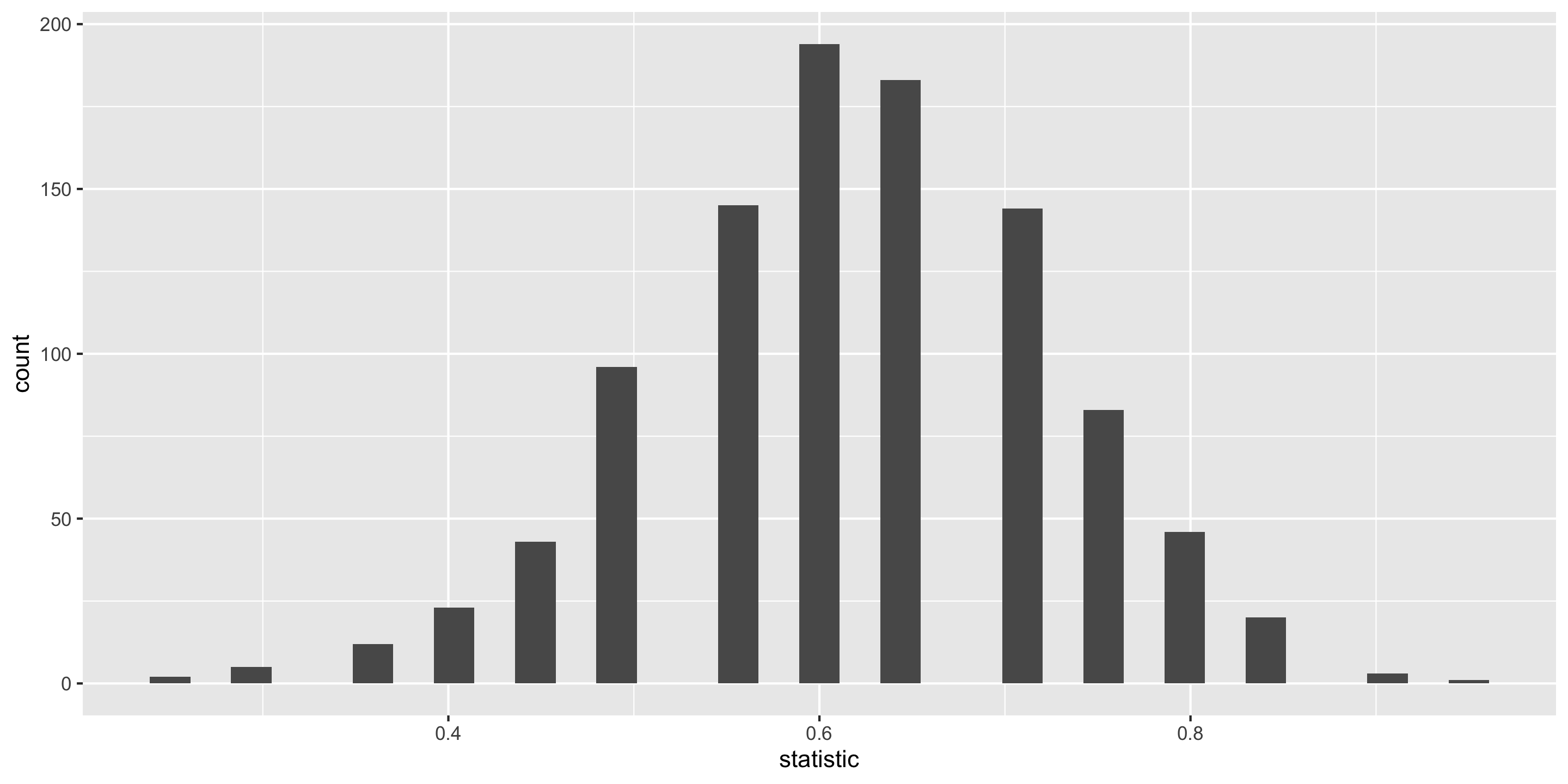
Bootstraping: Algorithm

How do we approximate the sampling distribution?

Bootstrap Distribution of a Sample Statistic:

  1. Take a sample of size \(n\) with replacement from the sample. Called a bootstrap sample.

  2. Compute the statistic on the bootstrap sample.

  3. Repeat 1 and 2 many (1000+) times.

Let’s Practice Generating Bootstrap Samples!

Example: In a recent study, 23 rats showed compassion that surprised scientists. Twenty-three of the 30 rats in the study freed another trapped rat in their cage, even when chocolate served as a distraction and even when the rats would then have to share the chocolate with their freed companion. (Rats, it turns out, love chocolate.) Rats did not open the cage when it was empty or when there was a stuffed animal inside, only when a fellow rat was trapped. We wish to use the sample to estimate the proportion of rats that show empathy in this way.

  • Parameter:

  • Statistic:

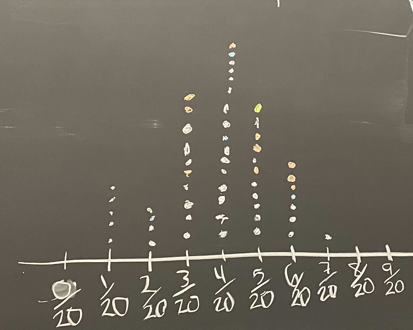
Use your 30 cards to take a bootstrap sample. (Make sure to appropriately label them first!)

Compute the bootstrap statistic and put it on the class dotplot.

Sampling Distribution Versus Bootstrap Distribution

  • Data needed:


  • Center:


  • Spread:

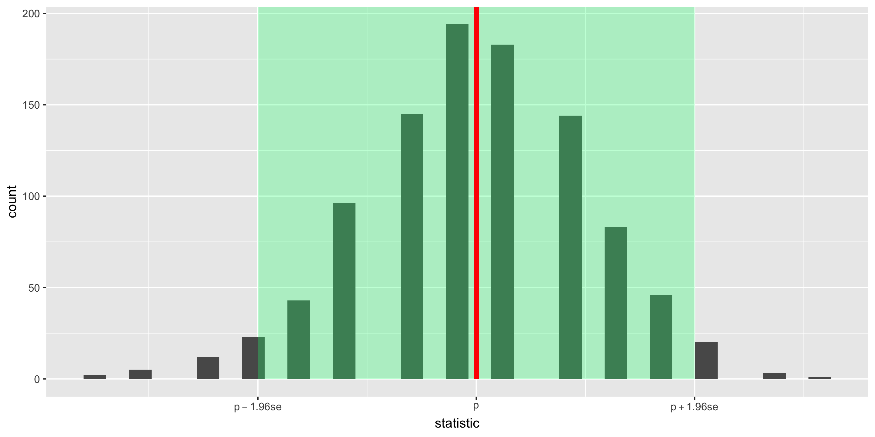
(Bootstrapped) Confidence Intervals

95% CI Form:

\[ \mbox{statistic} \pm 1.96 \times\mbox{SE} \]

We approximate \(\mbox{SE}\) with \(\widehat{\mbox{SE}}\) = the standard deviation of the bootstrapped statistics.

Caveats:

  • Assuming a random sample

  • Even with random samples, sometimes we get non-representative samples. Bootstrapping can’t fix that.

  • Assuming the bootstrap distribution is bell-shaped and symmetric

Bootstrapped Confidence Intervals

Two Methods

Assuming random sample and roughly bell-shaped and symmetric bootstrap distribution for both methods.

SE Method 95% CI:

\[ \mbox{statistic} \pm 1.96 \times\widehat{\mbox{SE}} \]

We approximate \(\mbox{SE}\) with \(\widehat{\mbox{SE}}\) = the standard deviation of the bootstrapped statistics.


Percentile Method CI:

If I want a P% confidence interval, I find the bounds of the middle P% of the bootstrap distribution.

How can we construct bootstrap distributions and bootstrapped CIs in R?

Load Packages and Data

library(tidyverse)
library(infer)
library(palmerpenguins)

Let’s return to the palmer penguins!

# Read in data
head(penguins)
# A tibble: 6 × 8
  species island    bill_length_mm bill_depth_mm flipper_length_mm body_mass_g
  <fct>   <fct>              <dbl>         <dbl>             <int>       <int>
1 Adelie  Torgersen           39.1          18.7               181        3750
2 Adelie  Torgersen           39.5          17.4               186        3800
3 Adelie  Torgersen           40.3          18                 195        3250
4 Adelie  Torgersen           NA            NA                  NA          NA
5 Adelie  Torgersen           36.7          19.3               193        3450
6 Adelie  Torgersen           39.3          20.6               190        3650
# ℹ 2 more variables: sex <fct>, year <int>

Estimation for a Single Mean

What is the average bill length \((\mu)\) of an Adelie penguin?

# Compute the summary statistic
x_bar <- penguins %>%
  drop_na(bill_length_mm) %>%
  specify(response = bill_length_mm) %>%
  calculate(stat = "mean")
x_bar
Response: bill_length_mm (numeric)
# A tibble: 1 × 1
   stat
  <dbl>
1  43.9
  • Why is our numerical quantity a mean and not a proportion or correlation here?

Estimation for a Single Mean

# Construct bootstrap distribution
bootstrap_dist <- penguins %>%
  drop_na(bill_length_mm) %>%
  specify(response = bill_length_mm) %>%
  generate(reps =  1000, type = "bootstrap") %>%
  calculate(stat = "mean")

# Look at bootstrap distribution
ggplot(data = bootstrap_dist, 
       mapping = aes(x = stat)) +
  geom_histogram(color = "white")

Estimation for a Single Mean – SE Method

# Get confidence interval
ci <- bootstrap_dist %>% 
  get_confidence_interval(type = "se", level = 0.95,
                          point_estimate = x_bar)
ci
# A tibble: 1 × 2
  lower_ci upper_ci
     <dbl>    <dbl>
1     43.3     44.5

Interpretation: The point estimate is 43.92mm. I am 95% confidence that the average bill length of Adelie penguins is between 43.33mm and 44.52mm.

Estimation for a Single Mean

# Visualize confidence interval
bootstrap_dist %>%
  visualize() +
  shade_confidence_interval(endpoints = ci)

Estimation for a Single Mean – Percentile Method

# Get confidence interval 
ci_95 <- bootstrap_dist %>% 
  get_confidence_interval(type = "percentile",
                          level = 0.95) 
ci_95
# A tibble: 1 × 2
  lower_ci upper_ci
     <dbl>    <dbl>
1     43.4     44.6

Estimation for Difference in Means

What is the difference in average bill length between Adelie penguins and Chinstrap penguins \((\mu_1 - \mu_2)\)?

# Compute the summary statistic
diff_x_bar <- penguins %>%
  drop_na(bill_length_mm) %>%
  filter(species %in% c("Adelie", "Chinstrap")) %>%
  specify(bill_length_mm ~ species) %>%
  calculate(stat = "diff in means")
diff_x_bar
Response: bill_length_mm (numeric)
Explanatory: species (factor)
# A tibble: 1 × 1
   stat
  <dbl>
1 -10.0
  • Why a difference in means?

Estimation for Difference in Means

# Construct bootstrap distribution
bootstrap_dist <-penguins %>%
  drop_na(bill_length_mm) %>%
  filter(species %in% c("Adelie", "Chinstrap")) %>%
  specify(bill_length_mm ~ species) %>%
  generate(reps =  1000, type = "bootstrap") %>%
  calculate(stat = "diff in means",
            order = c("Adelie", "Chinstrap"))

# Look at bootstrap distribution
ggplot(data = bootstrap_dist,
       mapping = aes(x = stat)) +
  geom_histogram(color = "white")

Estimation for Difference in Means – SE Method

# Get confidence interval 
ci_95 <- bootstrap_dist %>% 
  get_confidence_interval(type = "se", level = 0.95,
                          point_estimate = diff_x_bar) 
ci_95
# A tibble: 1 × 2
  lower_ci upper_ci
     <dbl>    <dbl>
1    -10.9    -9.16

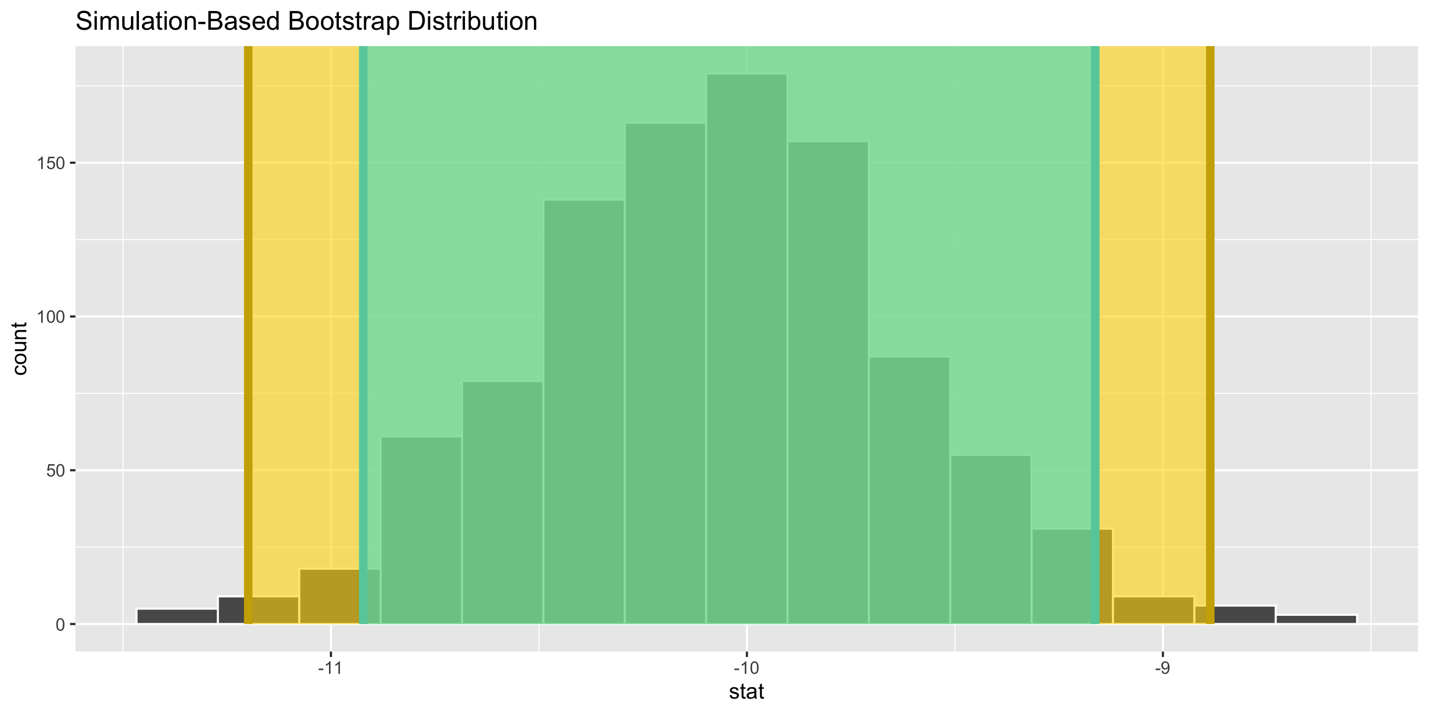
Interpretation: The point estimate is -10.04mm. I am 95% confidence that the difference in bill length between Adelie and Chinstrap penguins is, on average, between -10.92mm and -9.16mm.

Comparing CIs

ci_99 <- bootstrap_dist %>% 
  get_confidence_interval(type = "se", level = 0.99,
                          point_estimate = diff_x_bar)

bootstrap_dist %>%
  visualize() +
  shade_confidence_interval(endpoints = ci_99,
                            fill = "gold1",
                            color = "gold3") +
  shade_confidence_interval(endpoints = ci_95) 

  • Why construct a 95% CI versus a 99% CI?

Next time: Dig into the meaning of the word “confidence”!

Reminders

  • See you tomorrow and Friday for oral exams!
  • Have an excellent fall break!