More Hypothesis Testing

Grayson White

Math 141
Week 8 | Fall 2025

Announcements

Clarifying midterm makeup points.

Goals for Today

Learn the language of hypothesis testing (including p-values)
Practice framing research questions in terms of hypotheses

Learn how to generate null distributions
Use infer to conduct hypothesis tests in R

Hypothesis Testing Framework

Have two competing hypothesis:

Null Hypothesis \((H_o)\): Dull hypothesis, status quo, random chance, no effect…
Alternative Hypothesis \((H_a)\): (Usually) contains the researchers’ conjecture.

Must first take those hypotheses and translate them into statements about the population parameters so that we can test them with sample data.

Example:

\(H_o\): ESP doesn’t exist.

\(H_a\): ESP does exist.

Then translate into a statistical problem!

\(p\) =

\(H_o\):

\(H_a\):

Let’s Practice Setting up Hypotheses!

Example 1

Can a simple smile have an effect on punishment assigned following an infraction? In a 1995 study, Hecht and LeFrance examined the effect of a smile on the leniency of disciplinary action for wrongdoers. Participants in the experiment took on the role of members of a college disciplinary panel judging students accused of cheating. For each suspect, along with a description of the offense, a picture was provided with either a smile or neutral facial expression. A leniency score was calculated based on the disciplinary decisions made by the participants.

Write out \(H_o\) and \(H_a\) in terms of conjectures.

Write out \(H_o\) and \(H_a\) in terms of population parameters.

Make sure to first define the population parameter in the context of the problem.

02:00

Example 2

Can you tell if a mouse is in pain by looking at its facial expression? A recent study created a “mouse grimace scale” and tested to see if there was a positive correlation between scores on that scale and the degree of pain (based on injections of a weak and mildly painful solution). The study’s authors believe that if the scale applies to other mammals as well, it could help veterinarians test how well painkillers and other medications work in animals.

Write out \(H_o\) and \(H_a\) in terms of conjectures.

Write out \(H_o\) and \(H_a\) in terms of population parameters.

Make sure to first define the population parameter in the context of the problem.

02:00

Hypothesis Testing Framework

Flavors of hypotheses:

\(H_o\): parameter \(=\) null value
One of the following:
- \(H_a\): parameter \(\neq\) null value
- \(H_a\): parameter \(>\) null value
- \(H_a\): parameter \(<\) null value

Question: But doesn’t \(H_o\) sometimes represent \(\leq\) or \(\geq\)?

Hypothesis Testing Framework

Once you have set-up your hypotheses…

Collect data.
Assume \(H_o\) is correct.
Quantify the likelihood of the sample results using a test statistic.
- Test statistic: Numerical summary of the sample data
  - Often is equal to the sample statistic.
- Null distribution: Sampling distribution of the test statistic if the null hypothesis is true.

Question: How do we use the null distribution to quantify the likelihood of the sample results?

Null Distributions and P-Values

p-value = Probability of the observed test statistic or more extreme if \(H_o\) is true

More extreme = direction of \(H_a\)
Find the proportion of test statistics in the null distribution that are equal to or more extreme that the observed test statistic
- Let’s draw some pictures.

P-values and Conclusions

If the p-value is small, we have evidence for \(H_a\).
If the p-value is not small, we don’t have evidence for \(H_a\).
In your conclusions, focus on \(H_a\) (the hypothesis that stores the researchers’ conjecture).
Will discuss conclusions in more detail soon!
- For example, what do we mean by “small”?

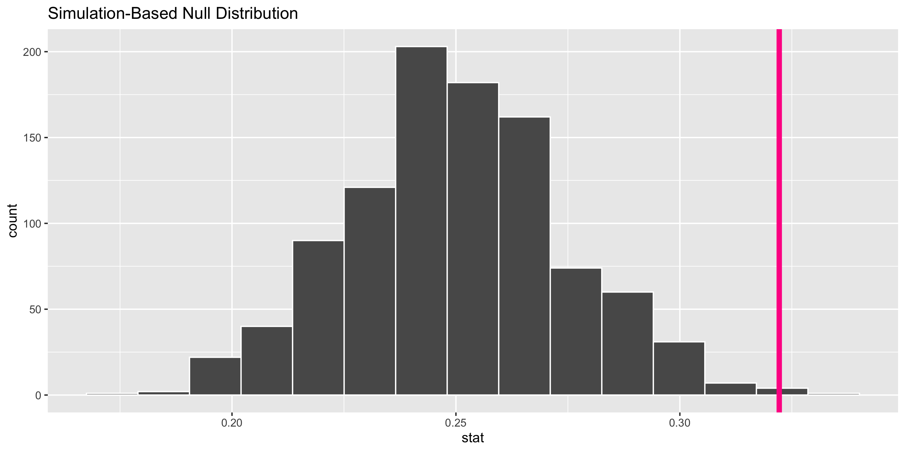
Generating Null Distributions

For the sample proportion in the ESP Example:

Steps:

Flip unfair coin (prop heads = 0.25) 329 times.
Compute proportion of heads.
Repeat 1 and 2 many times.

R code using the infer package:

library(infer)

# Construct data frame of sample results
esp <- data.frame(guess = c(rep("correct", 106),
                            rep("incorrect",
                                329 - 106)))

# Generate Null Distribution
null_dist <- esp %>%
  specify(response = guess, success = "correct") %>%
  hypothesize(null = "point", p = 0.25) %>%
  generate(reps = 1000, type = "draw") %>%
  calculate(stat ="prop")

For different variable types, we will need to move beyond using a coin to conceptualize the null distribution.

Hypothesis Testing in `R`

# Compute observed test statistic
test_stat <- esp %>%
  specify(response = guess, success = "correct") %>%
  calculate(stat ="prop")
test_stat

Response: guess (factor)
# A tibble: 1 × 1
   stat
  <dbl>
1 0.322

test_stat <- 106/329
test_stat

[1] 0.3221884

Hypothesis Testing in `R`

# Graph null distribution with test statistic
visualize(null_dist) +
  geom_vline(xintercept = test_stat,
             color = "deeppink", size = 2)

Hypothesis Testing in `R`

# Compute p-value
p_value <- null_dist %>%
  get_p_value(obs_stat = test_stat,
              direction = "right")
p_value

# A tibble: 1 × 1
  p_value
    <dbl>
1   0.003

Interpretation of \(p\)-value: If ESP doesn’t exist, the probability of observing 106 or more correct identifications out of 329 trials equals 0.003.

Conclusion: Since it is so unlikely (i.e., practically impossible) to have seen such unusual results if ESP doesn’t exist, these data suggest that ESP does exist.

Example

In 2005, the researchers Antonioli and Reveley posed the question “Does swimming with the dolphins help depression?” To investigate, they recruited 30 US subjects diagnosed with mild to moderate depression. Participants were randomly assigned to either the treatment group or the control group. Those in the treatment group went swimming with dolphins, while those in the control group went swimming without dolphins. After two weeks, each subject was categorized as “showed substantial improvement” or “did not show substantial improvement”.

Here’s a contingency table of improve and group.

dolphins %>%
  count(group, improve)

      group improve  n
1   Control      no 12
2   Control     yes  3
3 Treatment      no  5
4 Treatment     yes 10

\(H_o\):

\(H_a\):

How might we generate the null distribution for this scenario?

Dolphin Example

\(H_o\):

\(H_a\):

How might we generate the null distribution for this scenario?

Snapshot of the data:

      group improve
1   Control     yes
2 Treatment      no
3   Control      no
4 Treatment     yes
5   Control      no
6   Control      no
7 Treatment     yes
8   Control      no

Once you have your simulated null statistic, add it to the class dotplot.

Will finish the dolphin example on the next lab. Let’s return to the Palmer Penguins.

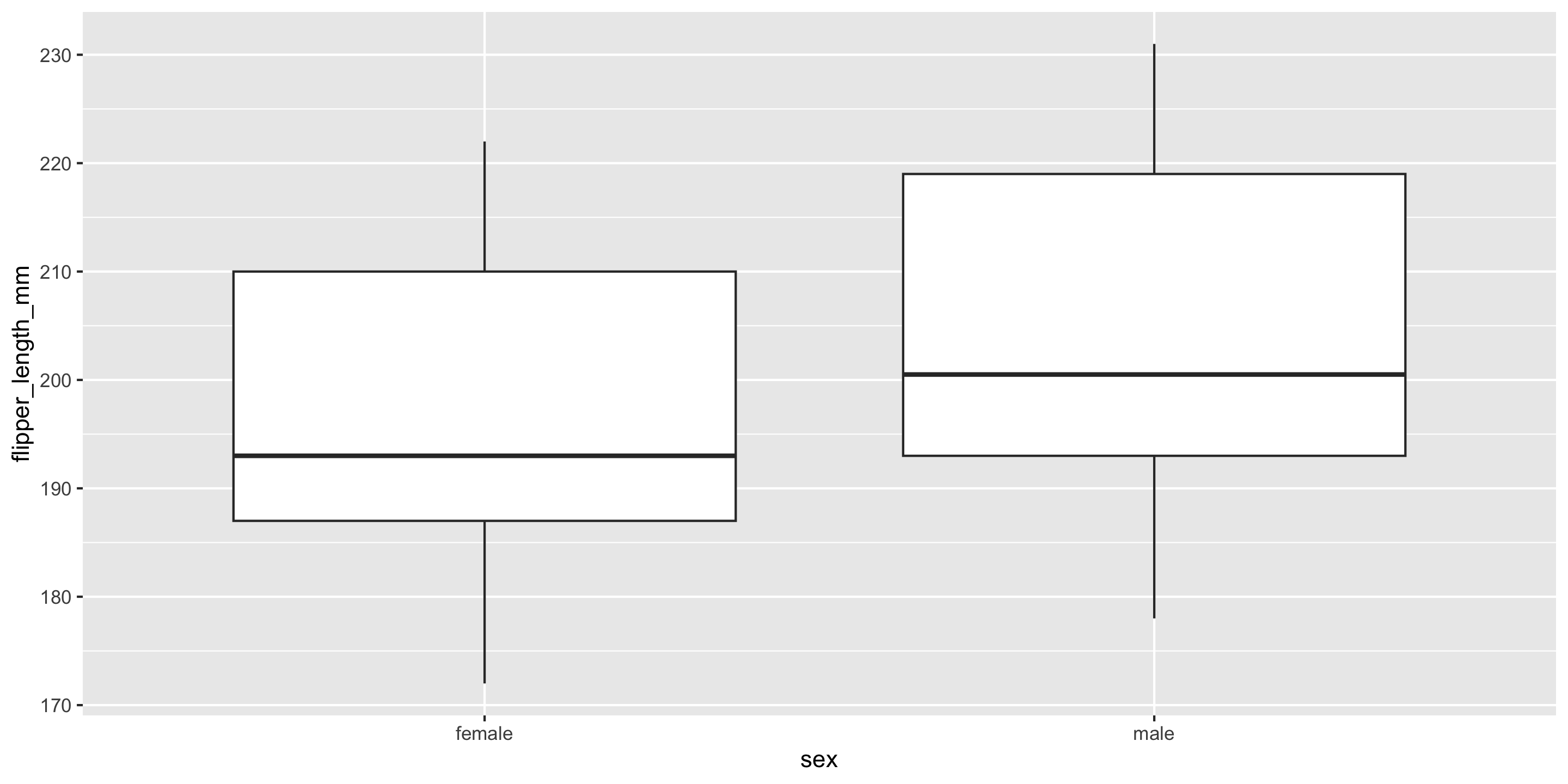
Penguins Example

Let’s return to the penguins data and ask if flipper length varies, on average, by the sex of the penguin.

Research Question: Does flipper length differ by sex?

Response Variable:

Explanatory Variable:

Statistical Hypotheses:

Exploratory Data Analysis

library(palmerpenguins)

penguins %>%
  drop_na(sex) %>%
ggplot(mapping = aes(x = sex,
                     y = flipper_length_mm)) +
  geom_boxplot()

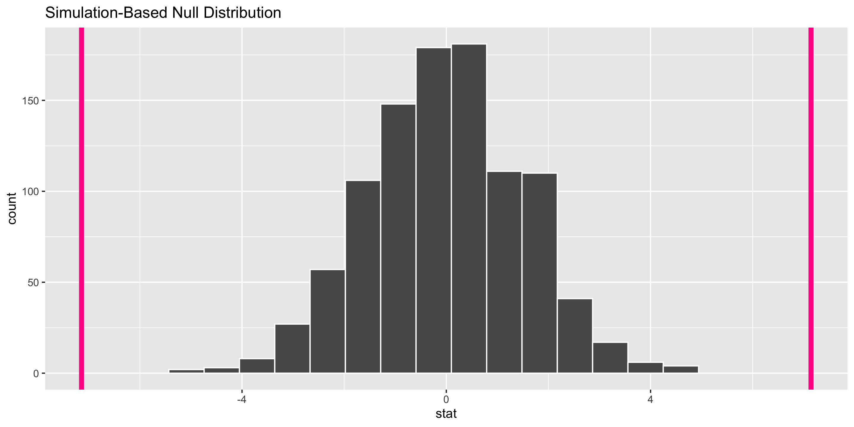
Two-Sided Hypothesis Test

# Compute observed test statistic
test_stat <- penguins %>%
  drop_na(sex) %>%
  specify(flipper_length_mm ~ sex) %>%
  calculate(stat ="diff in means",
            order = c("female", "male"))
test_stat

Response: flipper_length_mm (numeric)
Explanatory: sex (factor)
# A tibble: 1 × 1
   stat
  <dbl>
1 -7.14

# Generate null distribution 
null_dist <- penguins %>%
  drop_na(sex) %>%
  specify(flipper_length_mm ~ sex) %>%
  hypothesize(null = "independence") %>%
  generate(reps = 1000, type = "permute") %>%
  calculate(stat ="diff in means",
            order = c("female", "male"))

Two-Sided Hypothesis Test

# Graph null distribution with test statistic
visualize(null_dist) +
  geom_vline(xintercept = test_stat$stat,
             color = "deeppink", size = 2) +
  geom_vline(xintercept = abs(test_stat$stat),
             color = "deeppink", size = 2)

Two-Sided Hypothesis Test

# Compute p-value
p_value <- null_dist %>%
  get_p_value(obs_stat = test_stat,
              direction = "two_sided")
p_value

# A tibble: 1 × 1
  p_value
    <dbl>
1       0

Interpretation of \(p\)-value: If the mean flipper length does not differ by sex in the population, the probability of observing a difference in the sample means of at least 7.142316 mm (in magnitude) is equal to 0.

Conclusion: These data represent evidence that flipper length does vary by sex.

Hypothesis Testing Framework

Set-up hypotheses:
- Be able to express in words and in terms of parameters.
Collect data.
Assume \(H_o\) is correct.
Compute a p-value to quantify the likelihood of the sample results using a test statistic.

Next Class: A closer look at the conclusions of a hypothesis test

Announcements

Goals for Today

Hypothesis Testing Framework

Let’s Practice Setting up Hypotheses!

Example 1

Example 2

Hypothesis Testing Framework

Hypothesis Testing Framework

Null Distributions and P-Values

P-values and Conclusions

Generating Null Distributions

Hypothesis Testing in R

Hypothesis Testing in R

Hypothesis Testing in R

Example

Dolphin Example

Will finish the dolphin example on the next lab. Let’s return to the Palmer Penguins.

Penguins Example

Exploratory Data Analysis

Two-Sided Hypothesis Test

Two-Sided Hypothesis Test

Two-Sided Hypothesis Test

Hypothesis Testing Framework

Next Class: A closer look at the conclusions of a hypothesis test

Hypothesis Testing in `R`

Hypothesis Testing in `R`

Hypothesis Testing in `R`