Some logistics on Wednesday: (Written) midterm corrections, final exam info
Goals for Today
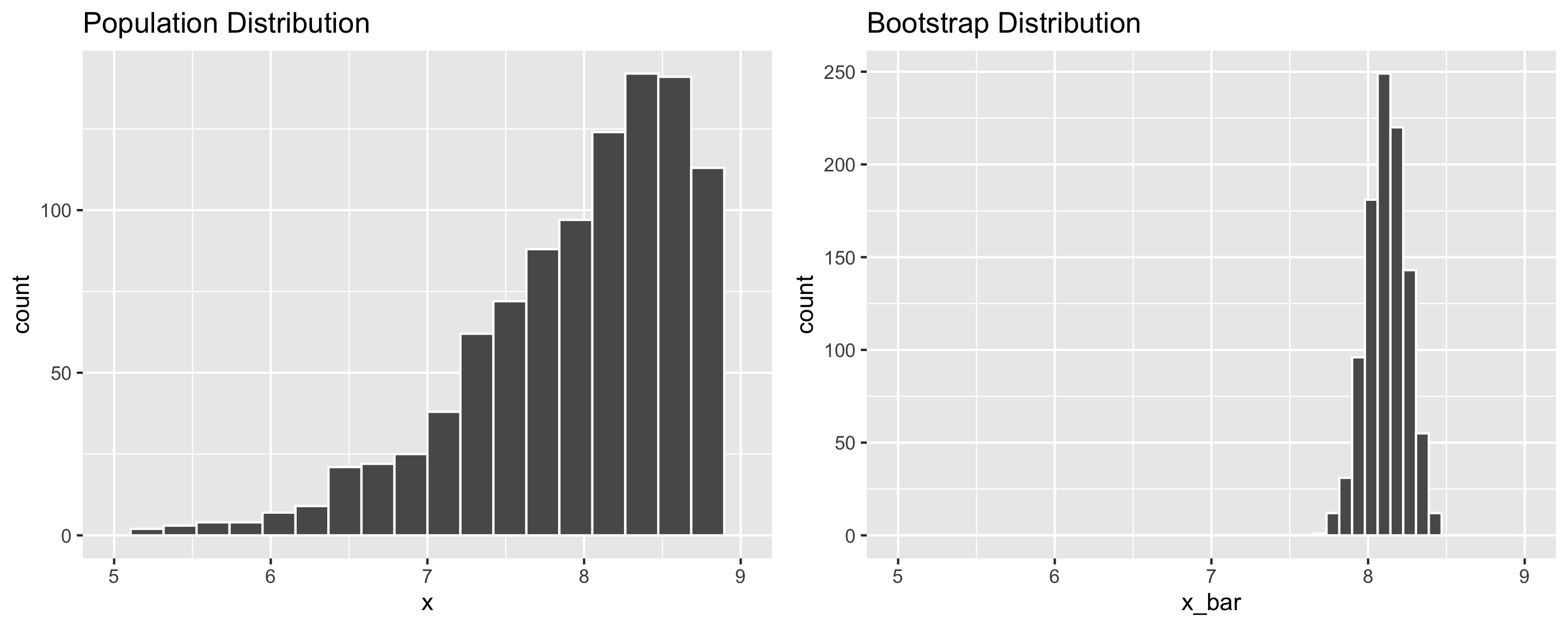
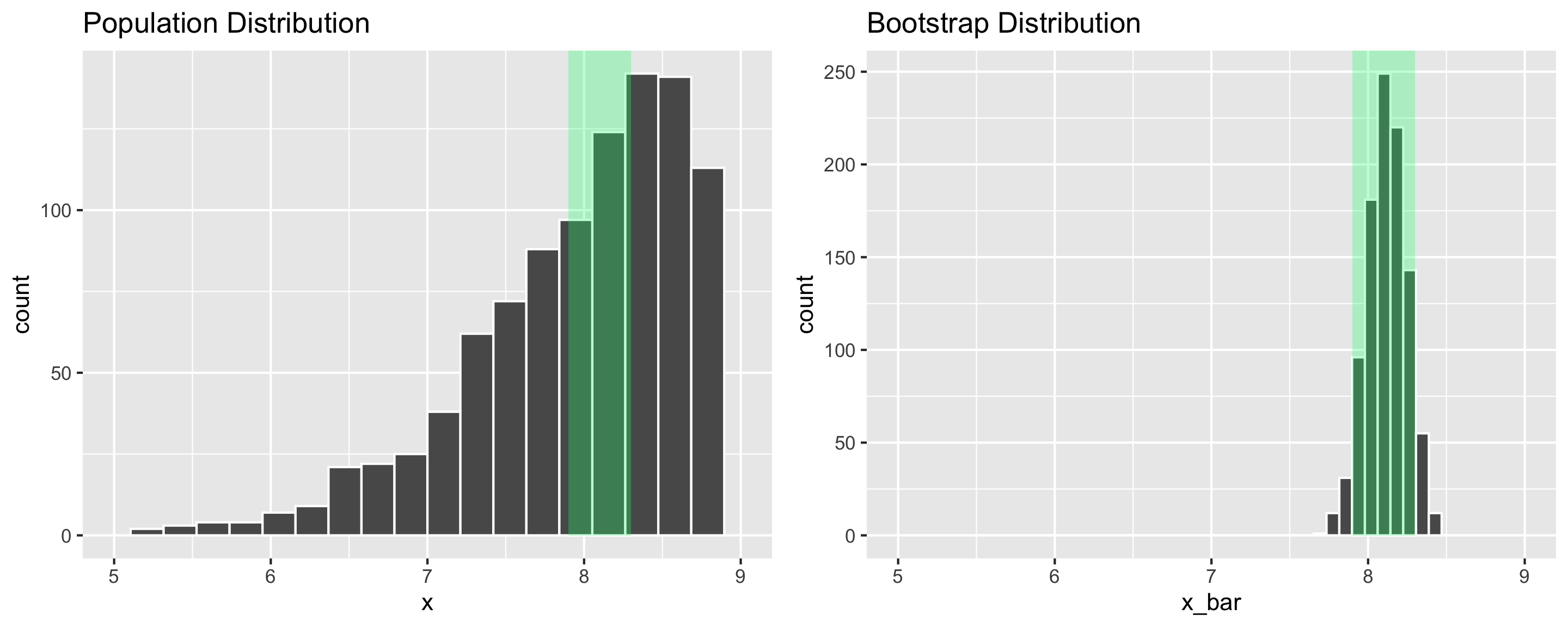
Recall ideas about the sampling distribution and bootstrapping
Bootstrapping in R
Learn more about confidence intervals and compute them in R
Review Discussion: Sampling distributions and bootstrapping
Confidence Intervals
Recall that a confidence interval is an interval of plausible values for a parameter.
Form: \(\mbox{statistic} \pm \mbox{Margin of Error}\)
Question: How do we find the Margin of Error (ME)?
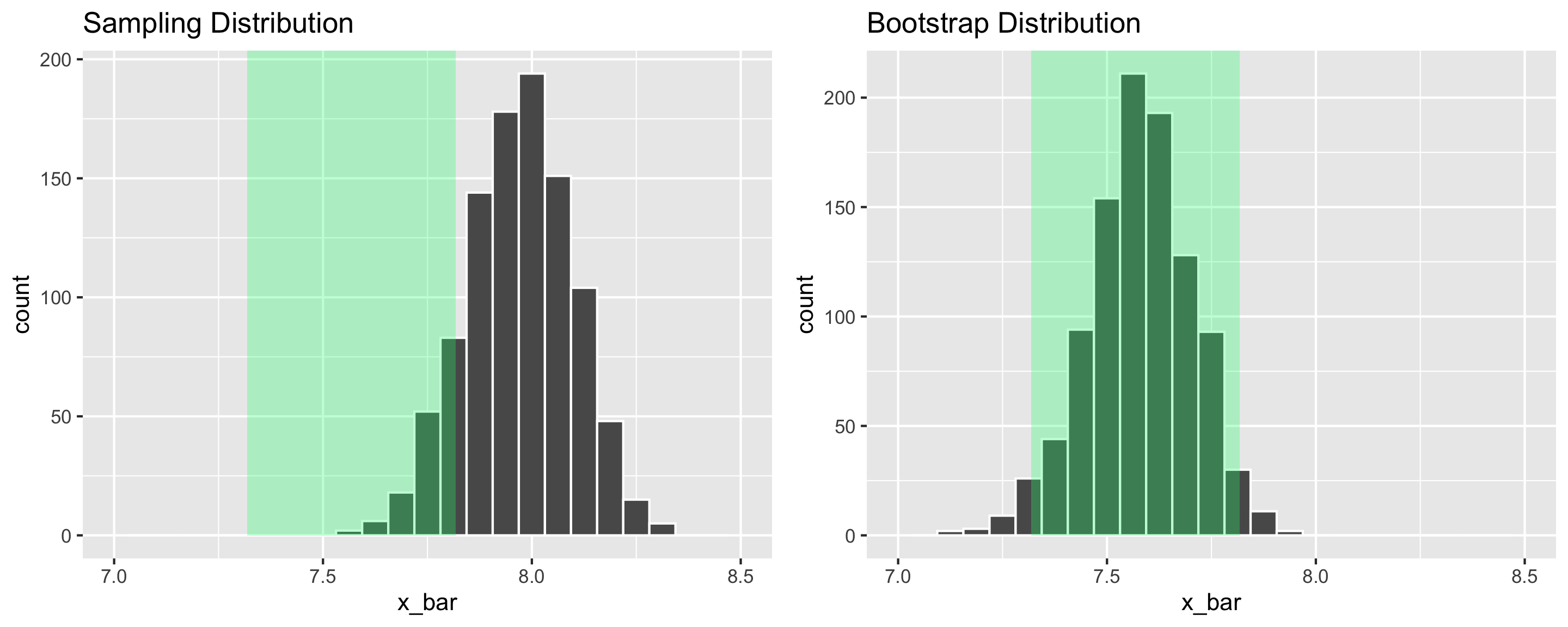
Answer: If the sampling distribution of the statistic is approximately bell-shaped and symmetric, then a statistic will be within 1.96 SEs of the parameter for 95% of the samples.
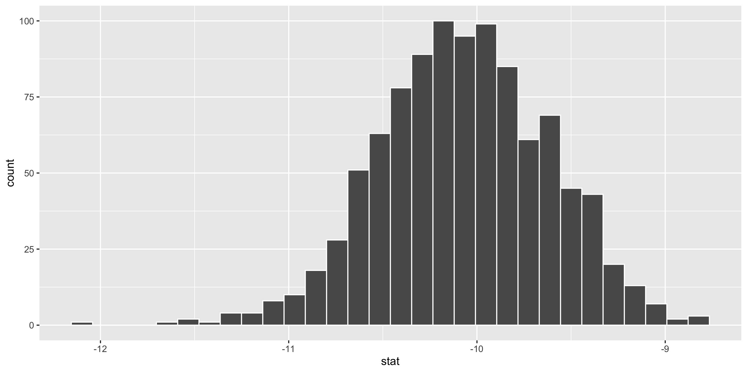
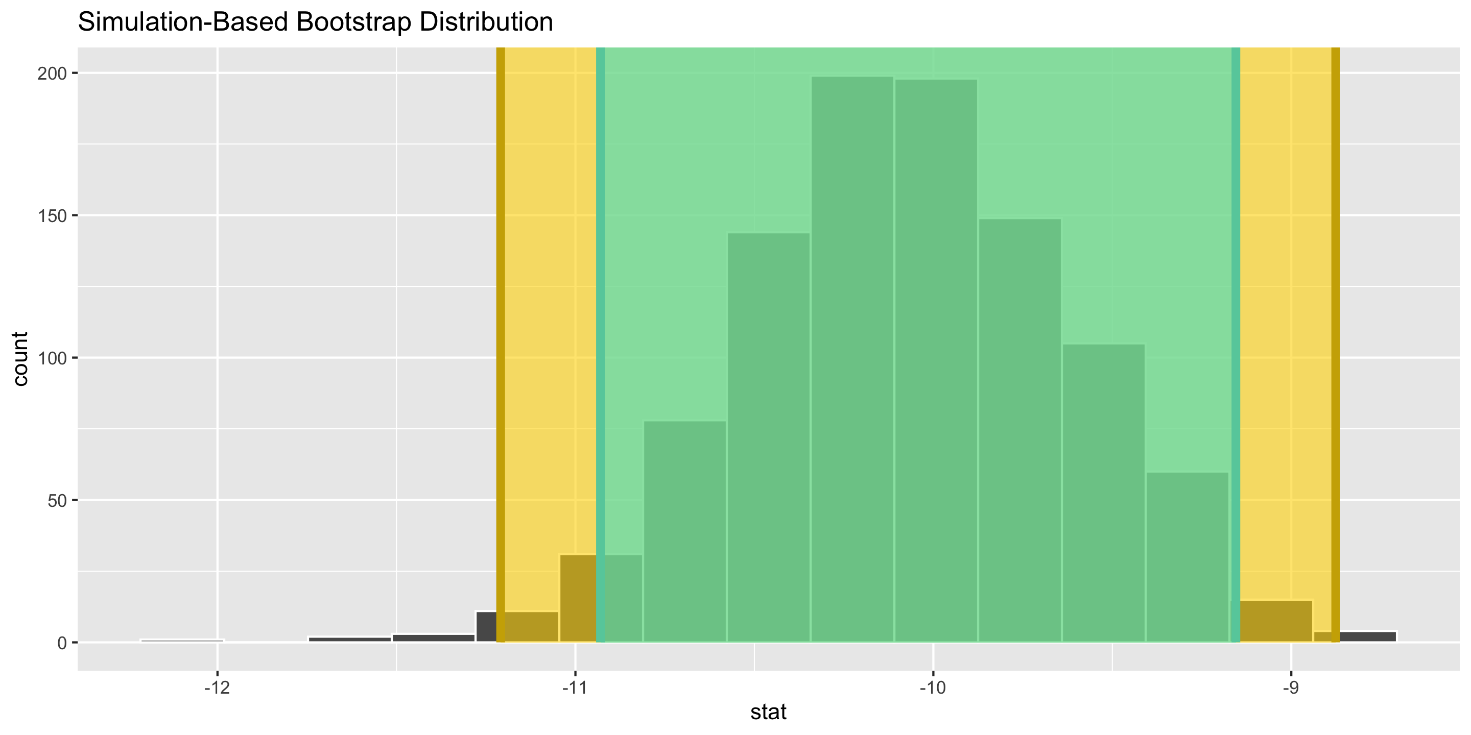
Interpretation: The point estimate is -10.04mm. I am 95% confident that the true average difference in bill length between Adelie and Chinstrap penguins is between -10.93mm and -9.15mm.
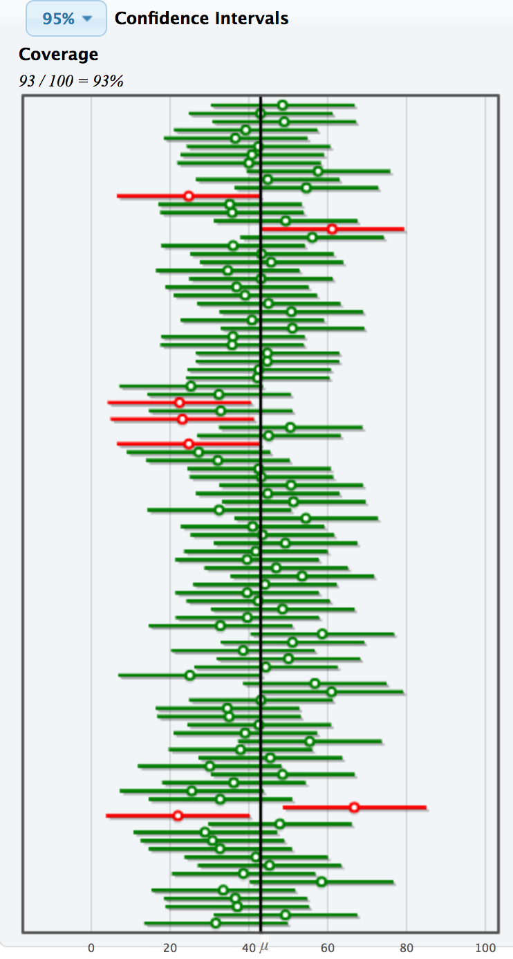
Confidence level = success rate of the method under repeated sampling
How do I know if my ONE CI successfully contains the true value of the parameter?
As we increase the confidence level, what happens to the width of the interval?
As we increase the sample size, what happens to the width of the interval?
As we increase the number of bootstrap samples we take, what happens to the width of the interval?
Interpreting Confidence Intervals
Example: Estimating average household income before taxes in the US
SE Method Formula:
\[
\mbox{statistic} \pm{\mbox{ME}}
\]
# A tibble: 1 × 4
  statistic    ME  lower  upper
      <dbl> <dbl>  <dbl>  <dbl>
1    62409. 1959. 60521. 64439.
“The margin of [sampling] error can be described as the ‘penalty’ in precision for not talking to everyone in a given population. It describes the range that an answer likely falls between if the survey had reached everyone in a population, instead of just a sample of that population.” – Courtney Kennedy, Director of Survey Research at Pew Research Center
CI = interval of plausible values for the parameter
Safe interpretation: I am P% confident that {insert what the parameter represents in context} is between {insert lower bound} and {insert upper bound}.
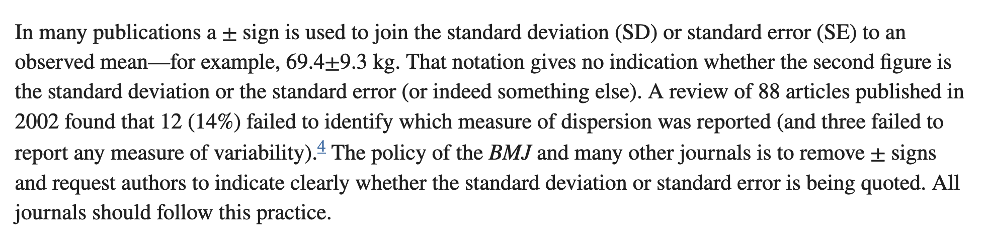
Caution: Intervals in the wild
Statement in an article for The BMJ (British Medical Journal):
Confidence Interval Misunderstandings
Misunderstanding 1
Suppose we wish to estimate the number of hours a Reed student sleeps on a typical night. We obtain the following 95% confidence interval: \((7.86, 8.34)\)
A 95% confidence interval does not contain 95% of observations in the population.
Misunderstanding 1
Suppose we wish to estimate the number of hours a Reed student sleeps on a typical night. We obtain the following 95% confidence interval: \((7.86, 8.34)\)
A 95% confidence interval does not contain 95% of observations in the population.
Saying that 95% of all Reed students sleep between 7.86 and 8.34 hours should just feel wrong. That’s a pretty narrow interval!
Misunderstanding 2
A 95% confidence interval does not mean that 95% of all sample means fall within the given range.
Misunderstanding 2
A 95% confidence interval does not mean that 95% of all sample means fall within the given range.
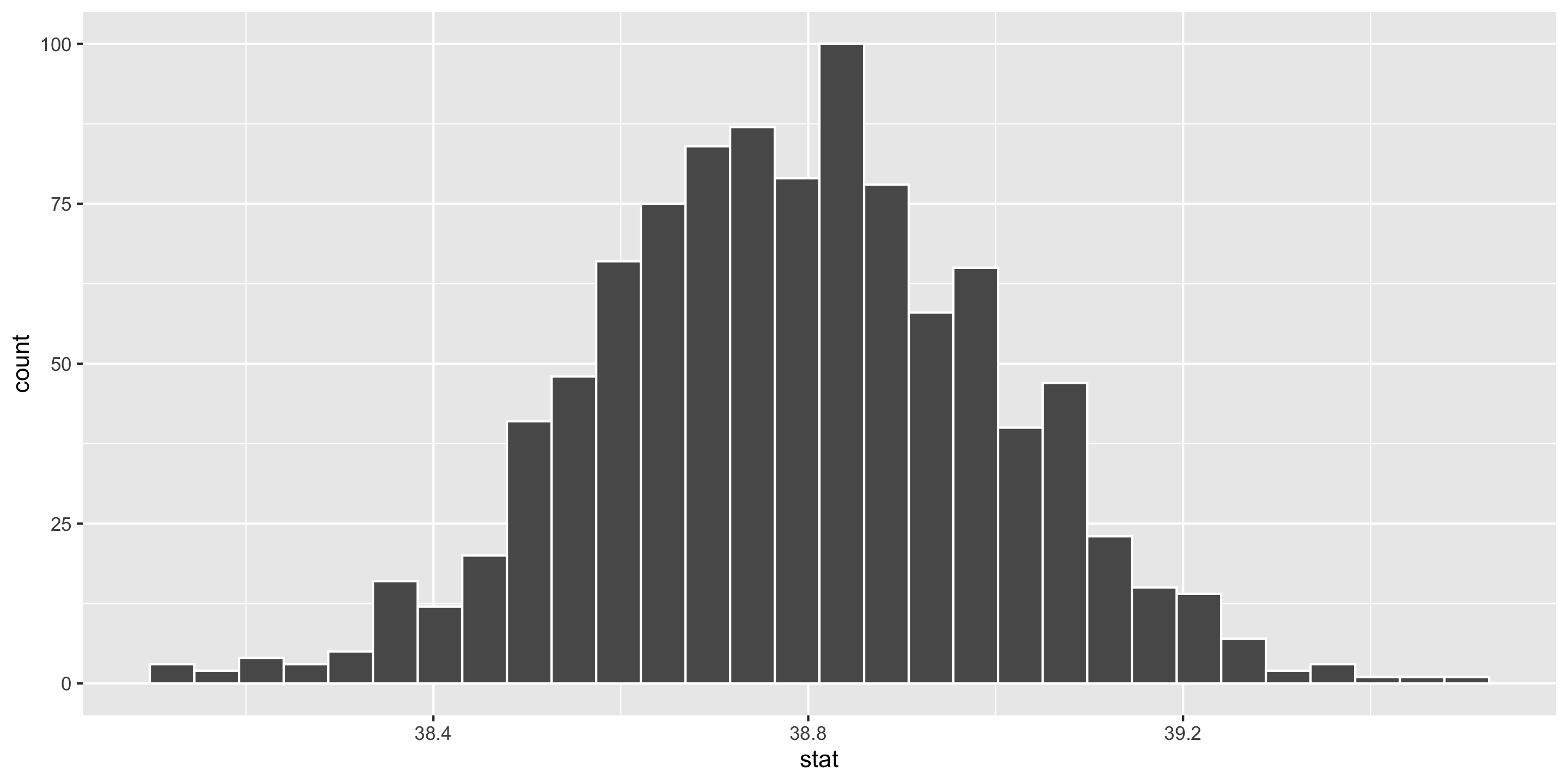
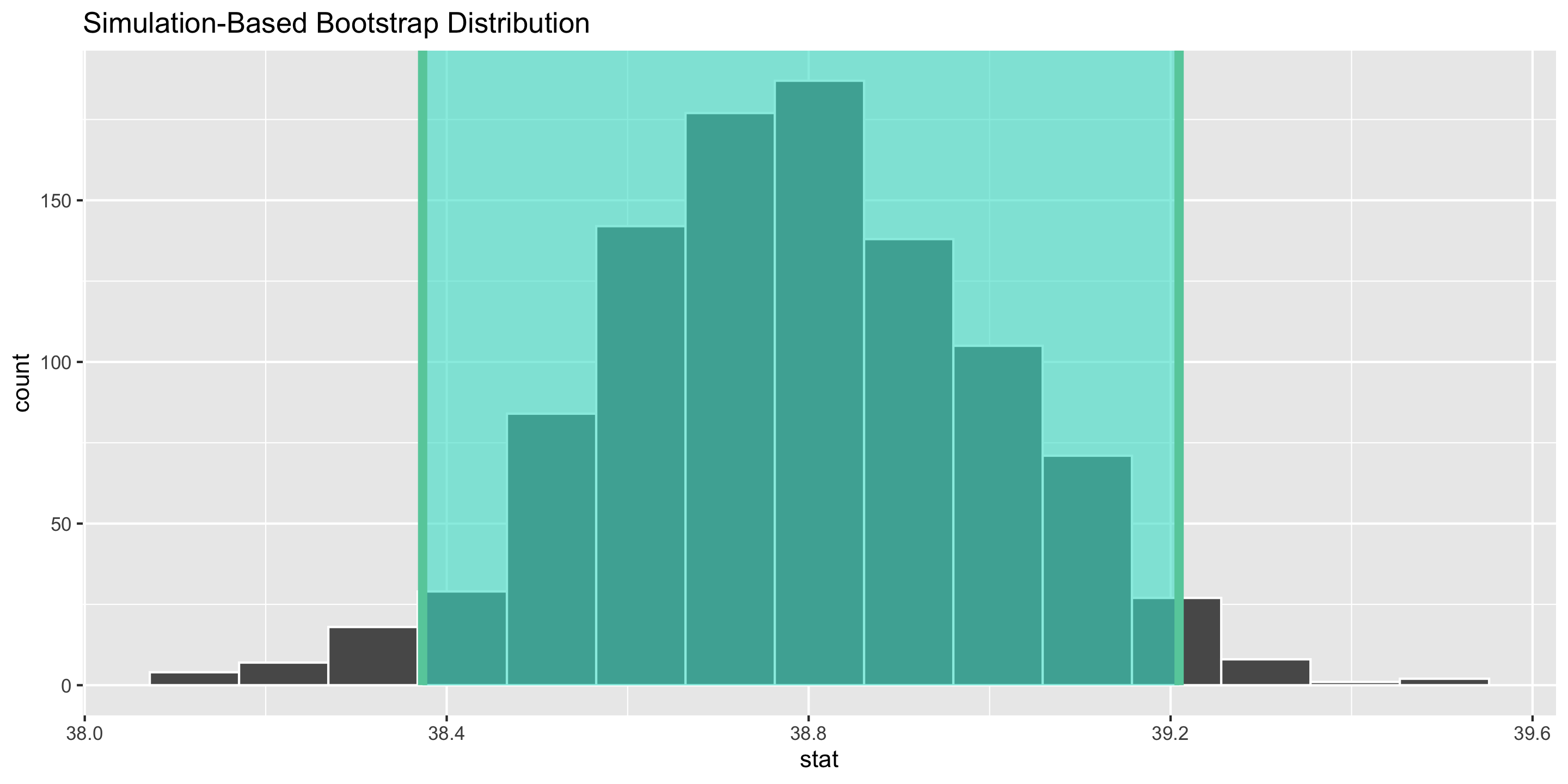
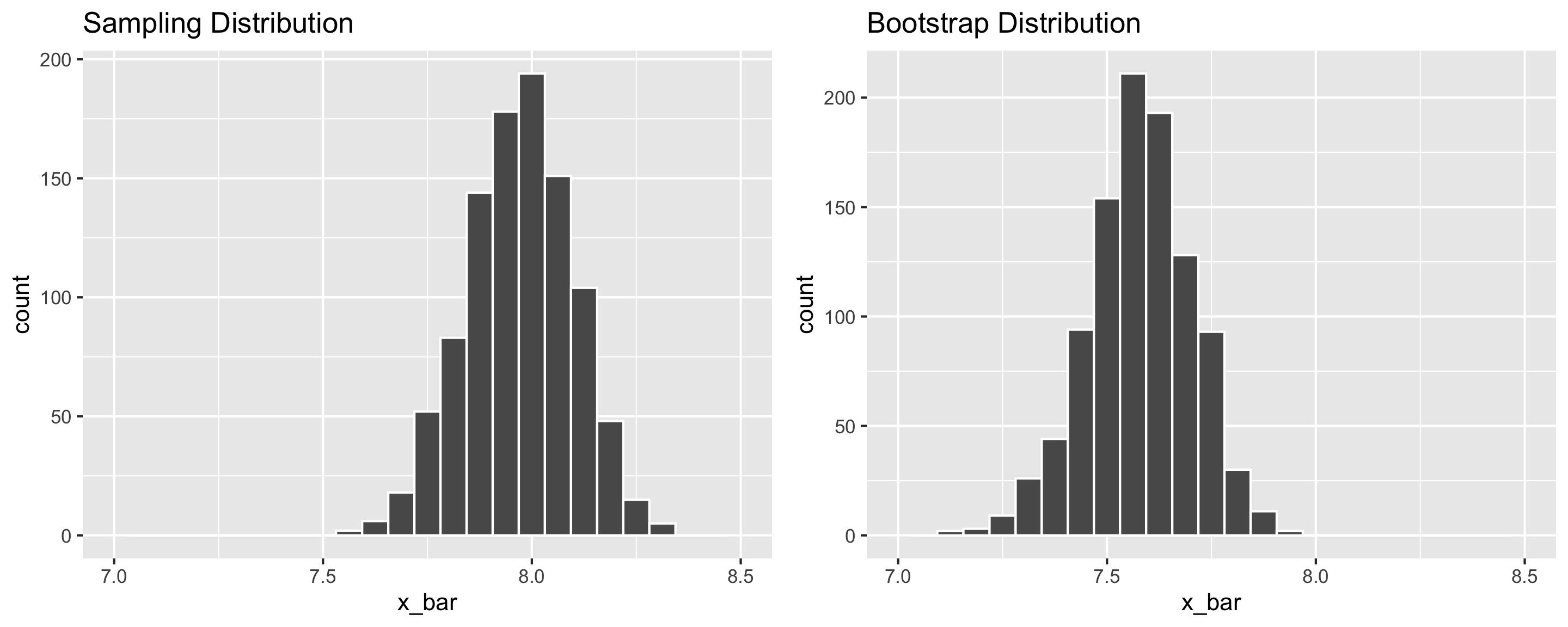
Q: Why do the sampling distribution and bootstrap distribution look different?
Misunderstanding 3
Given a 95% confidence interval, Do Not Say: “There is a 95% chance that the true parameter falls within my interval.”
Once we take a sample and calculate a confidence interval, there’s no more randomness!
The interval either does or doesn’t contain the (unknown) parameter.
This may seem like arguing over semantics – but it’s an important distinction!
Instead, say either:
“If we were to take many samples and calculate a confidence interval for each, 95% of them would contain the true parameter”
“We are 95% confident that the true parameter is in our confidence interval”