      group improve  n
1   Control      no 12
2   Control     yes  3
3 Treatment      no  5
4 Treatment     yes 10
More Hypothesis Testing
Grayson White
Math 141
Week 9 | Fall 2025
Goals for Today
- Practice framing research questions in terms of hypotheses
- Work through more Hypothesis testing examples
- Decisions in a hypothesis test
- Types of errors
- The power of a hypothesis test
Hypothesis Testing Framework
Have two competing hypothesis:
Null Hypothesis \((H_o)\): Dull hypothesis, status quo, random chance, no effect…
Alternative Hypothesis \((H_a)\): (Usually) contains the researchers’ conjecture.
Must first take those hypotheses and translate them into statements about the population parameters so that we can test them with sample data.
Example:
\(H_o\): ESP doesn’t exist.
\(H_a\): ESP does exist.
Then translate into a statistical problem!
\(p\) =
\(H_o\):
\(H_a\):
New Example: Swimming with Dolphins
In 2005, the researchers Antonioli and Reveley posed the question “Does swimming with the dolphins help depression?” To investigate, they recruited 30 US subjects diagnosed with mild to moderate depression. Participants were randomly assigned to either the treatment group or the control group. Those in the treatment group went swimming with dolphins, while those in the control group went swimming without dolphins. After two weeks, each subject was categorized as “showed substantial improvement” or “did not show substantial improvement”.
Here’s a contingency table of improve and group.
\(H_o\):
\(H_a\):
How might we generate the null distribution for this scenario?
Dolphin Example
\(H_o\):
\(H_a\):
How might we generate the null distribution for this scenario?
Snapshot of the data:
      group improve
1   Control     yes
2 Treatment      no
3   Control      no
4 Treatment     yes
5   Control      no
6   Control      no
7 Treatment     yes
8   Control      no
Once you have your simulated null statistic, add it to the class dotplot.
Will finish the dolphin example on the next lab. Let’s return to the Palmer Penguins.

Penguins Example
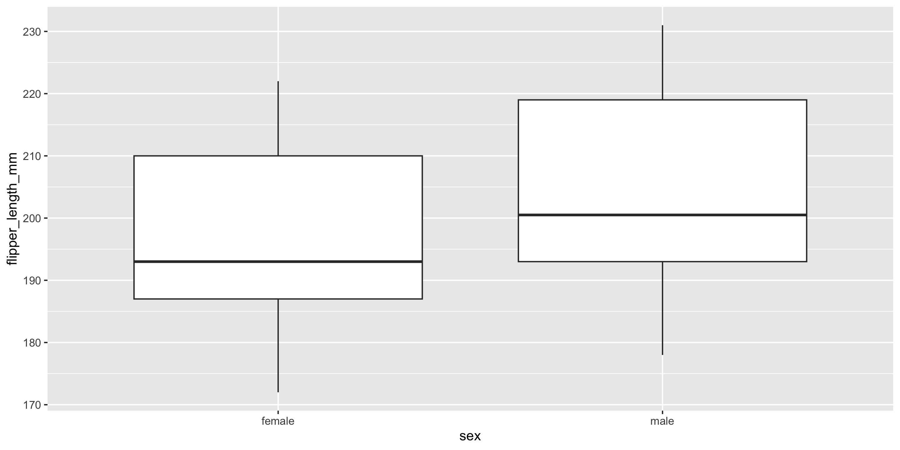
Let’s return to the penguins data and ask if flipper length varies, on average, by the sex of the penguin.
Research Question: Does flipper length differ by sex?
Response Variable:
Explanatory Variable:
Statistical Hypotheses:
Exploratory Data Analysis
Two-Sided Hypothesis Test
Response: flipper_length_mm (numeric)
Explanatory: sex (factor)
# A tibble: 1 × 1
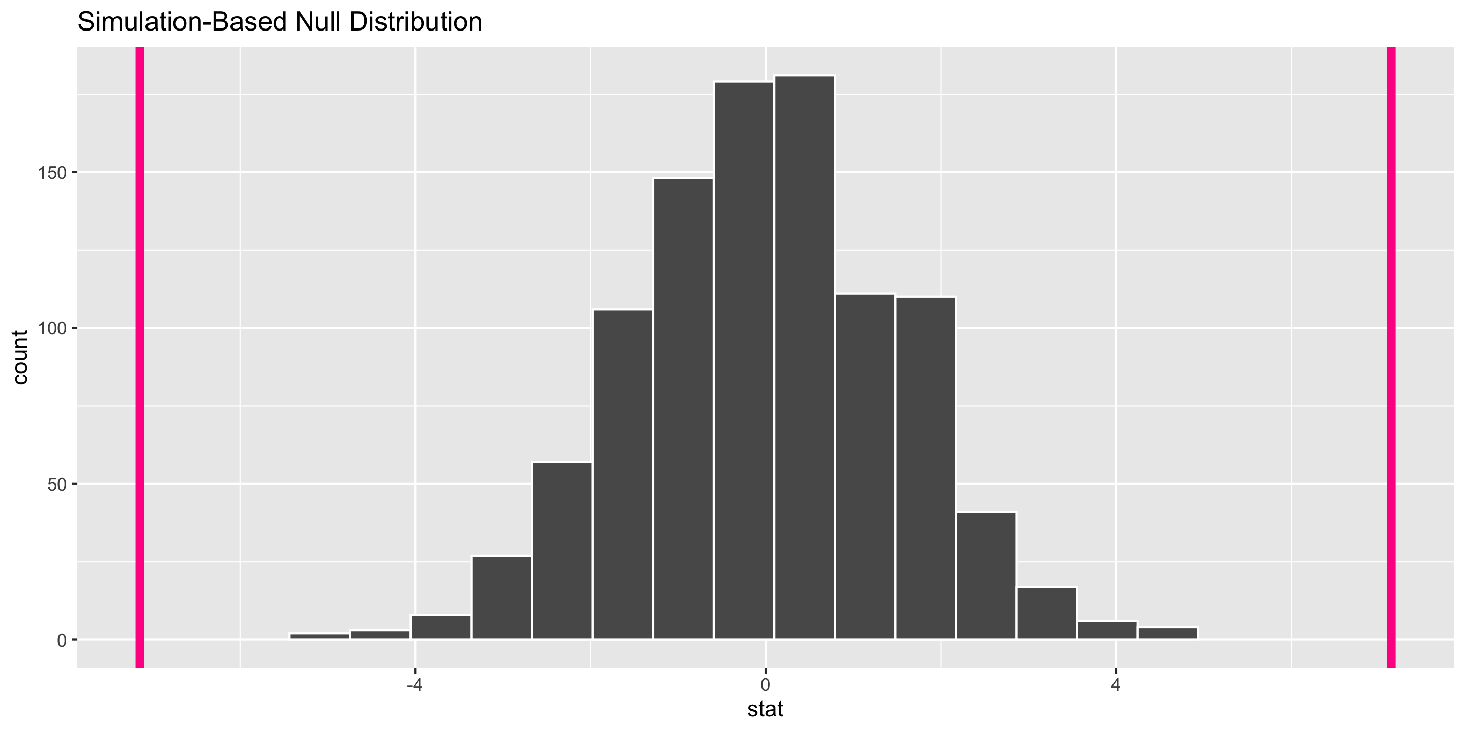
stat
<dbl>
1 -7.14Two-Sided Hypothesis Test
Two-Sided Hypothesis Test
# A tibble: 1 × 1
  p_value
    <dbl>
1       0
Interpretation of \(p\)-value: If the mean flipper length does not differ by sex in the population, the probability of observing a difference in the sample means of at least 7.14 mm (in magnitude) is equal to 0.
Conclusion: These data represent evidence that flipper length does vary by sex.
Hypothesis Testing Framework
Set-up hypotheses:
- Be able to express in words and in terms of parameters.
Collect data.
Assume \(H_o\) is correct.
Compute a p-value to quantify the likelihood of the sample results using a test statistic.
Draw a conclusion about the alternative hypothesis.
Now: A closer look at the conclusions of a hypothesis test
Hypothesis Testing: Decisions, Decisions
Once you get to the end of a hypothesis test you make one of two decisions:
- P-value is small.
- I have evidence for \(H_a\). Reject \(H_o\).
- P-value is not small.
- I don’t have evidence for \(H_a\). Fail to reject \(H_o\).
Sometimes we make the correct decision. Sometimes we make a mistake.
Hypothesis Testing: Decisions, Decisions
Let’s create a table of potential outcomes.
\(\alpha\) = prob of Type I error under repeated sampling = prob reject \(H_o\) when it is true
\(\beta\) = prob of Type II error under repeated sampling = prob fail to reject \(H_o\) when \(H_a\) is true.
Hypothesis Testing: Decisions, Decisions
Typically set \(\alpha\) level beforehand.
Use \(\alpha\) to determine “small” for a p-value.
- P-value
issmall\(< \alpha\).- I have evidence for \(H_a\). Reject \(H_o\).
- P-value
isnotsmall\(\geq \alpha\).- I don’t have evidence for \(H_a\). Fail to reject \(H_o\).
Hypothesis Testing: Decisions, Decisions
Question: How do I select \(\alpha\)?
Will depend on the convention in your field.
Want a small \(\alpha\) and a small \(\beta\). But they are related.
- The smaller \(\alpha\) is the larger \(\beta\) will be.
Choose a lower \(\alpha\) (e.g., 0.01, 0.001) when the Type I error is worse and a higher \(\alpha\) (e.g., 0.1) when the Type II error is worse.
Can’t easily compute \(\beta\). Why?
One more important term:
- Power = probability reject \(H_o\) when the alternative is true.