
Computing Power
Grayson White
Math 141
Week 9 | Fall 2025
Example
Suppose we have a baseball player who has been a 0.250 career hitter who suddenly improves to be a 0.333 hitter. He wants a raise but needs to convince his manager that he has genuinely improved. The manager offers to examine his performance in 20 100 at-bats.
What will happen to the power of the test if we increase the sample size?
Increasing the sample size increases the power.
When \(\alpha\) is set to \(0.05\) and the sample size is now 100, the power of this test is 0.57.
Example
Suppose we have a baseball player who has been a 0.250 career hitter who suddenly improves to be a 0.333 hitter. He wants a raise but needs to convince his manager that he has genuinely improved. The manager offers to examine his performance in 20 100 at-bats.
What will happen to the power of the test if we increase \(\alpha\) to 0.1?
- Increasing \(\alpha\) increases the power.
- Decreases \(\beta\).
- When \(\alpha\) is set to \(0.1\) and the sample size is 100, the power of this test is 0.65.
Example
Suppose we have a baseball player who has been a 0.250 career hitter who suddenly improves to be a 0.333 0.400 hitter. He wants a raise but needs to convince his manager that he has genuinely improved. The manager offers to examine his performance in 20 100 at-bats.
What will happen to the power of the test if he is an even better player?
Effect size: Difference between true value of the parameter and null value.
- Often standardized.
Increasing the effect size increases the power.
When \(\alpha\) is set to \(0.1\), the sample size is 100, and the true probability of hitting the ball is 0.4, the power of this test is 0.95.
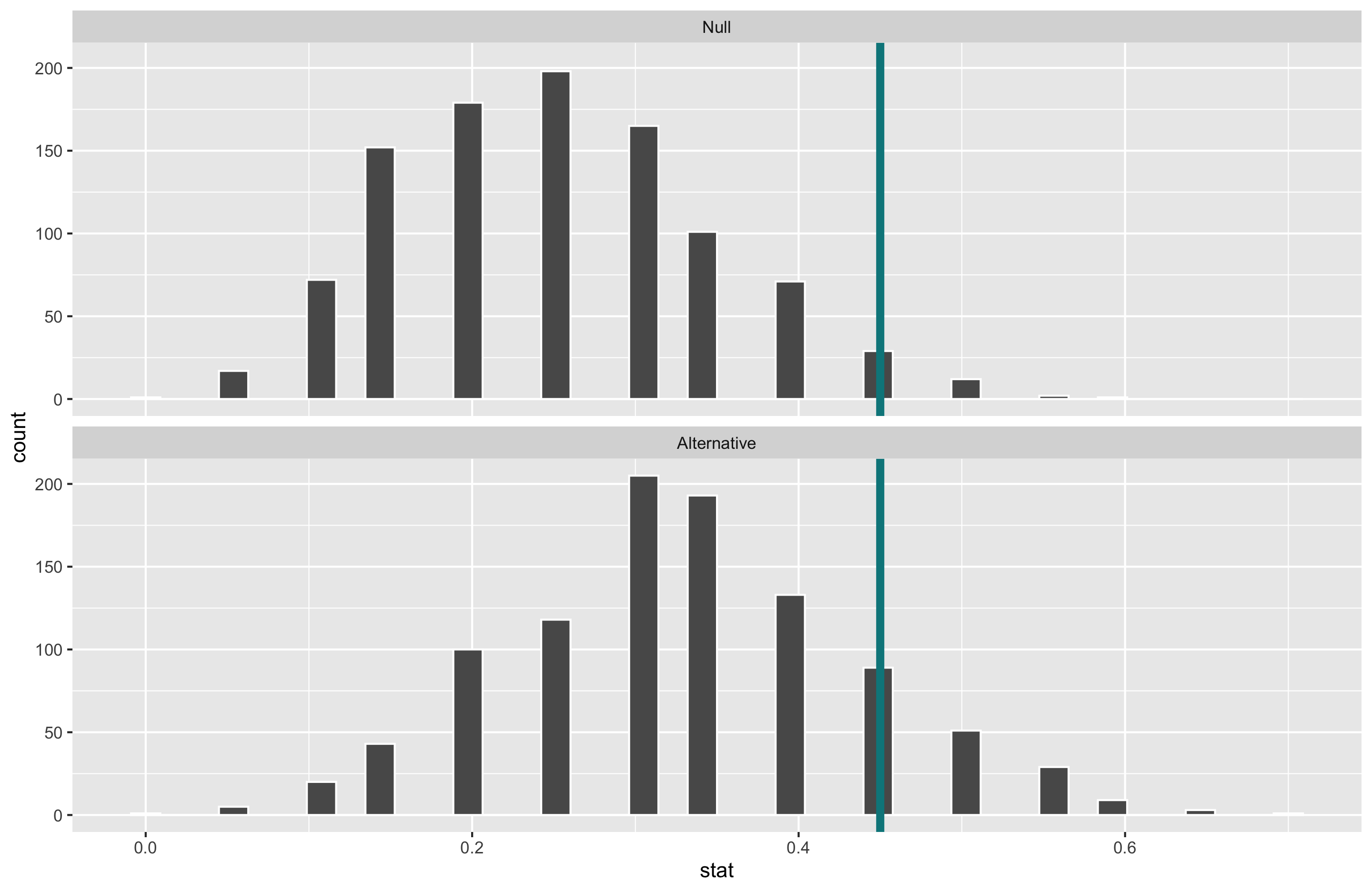
Computing Power
- Generate a null distribution:
# Create a dummy dataset with the correct sample size
dat <- data.frame(at_bats = c(rep("hit", 80),
                              rep("miss", 20)))


null <- dat %>%
  specify(response = at_bats, success = "hit") %>%
  hypothesize(null = "point", p = 0.25) %>%
  generate(reps = 1000, type = "draw") %>%
  calculate(stat = "prop")

ggplot(data = null, mapping = aes(x = stat)) +
  geom_histogram(bins = 27, color = "white")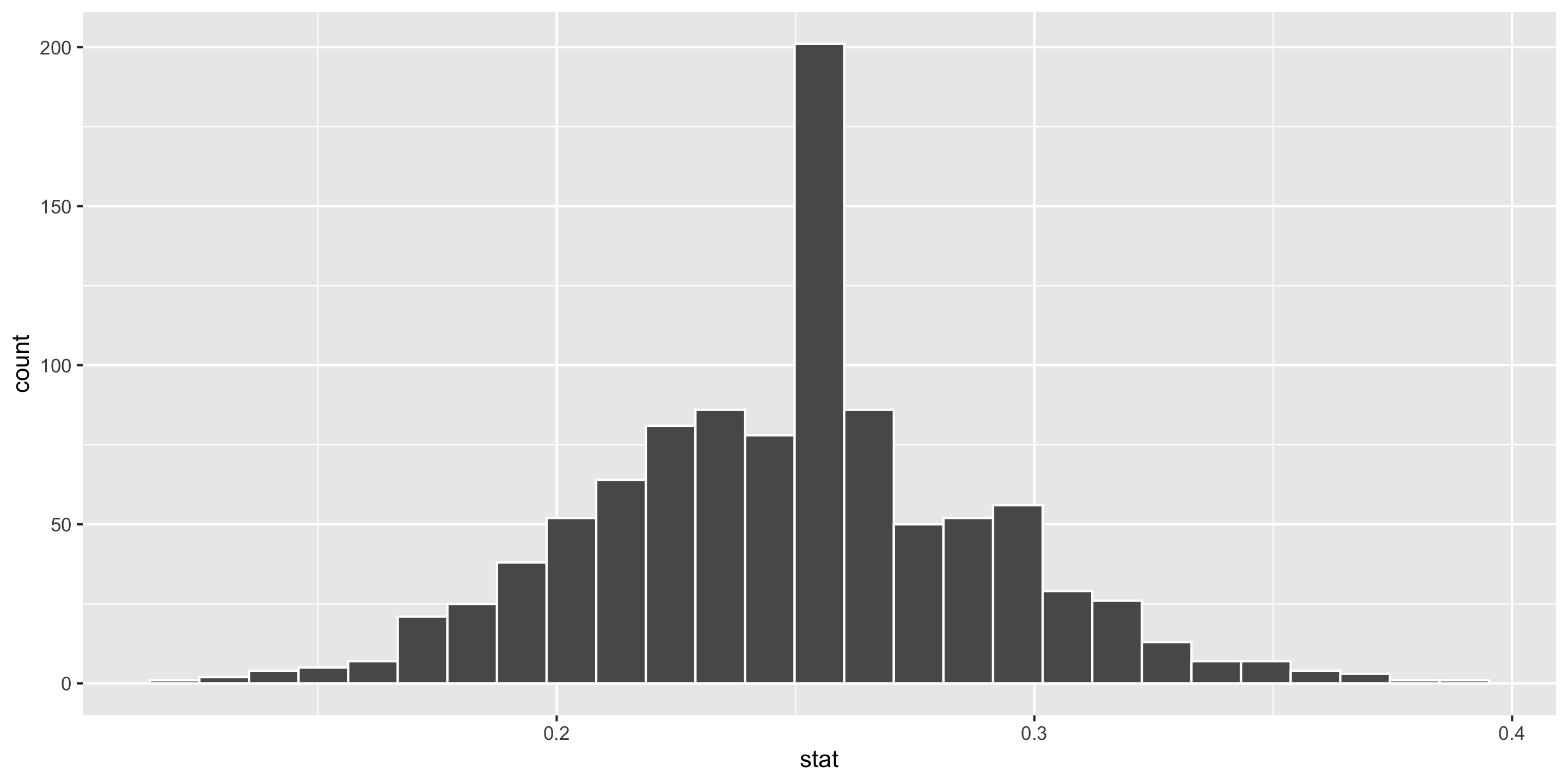
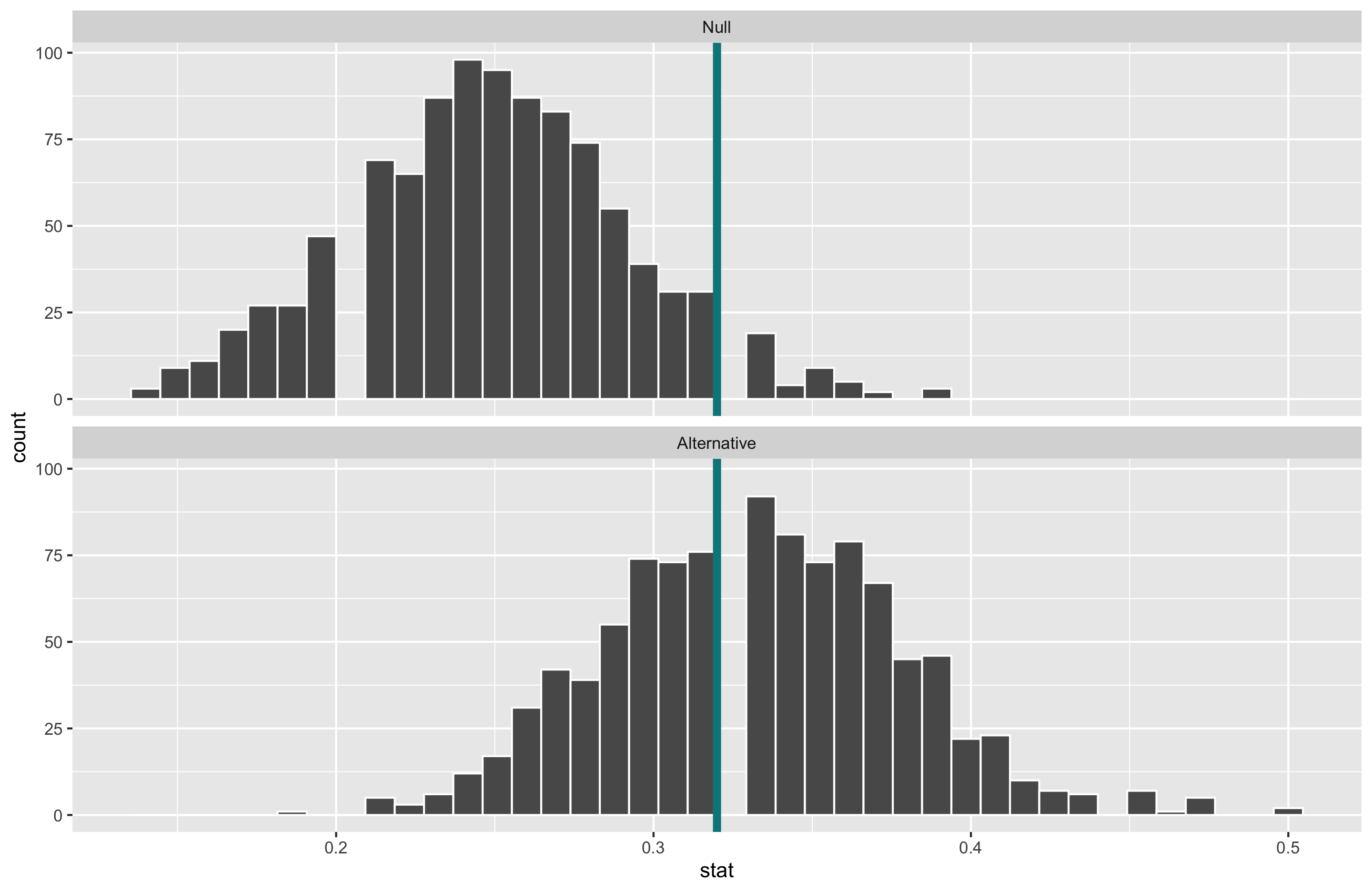
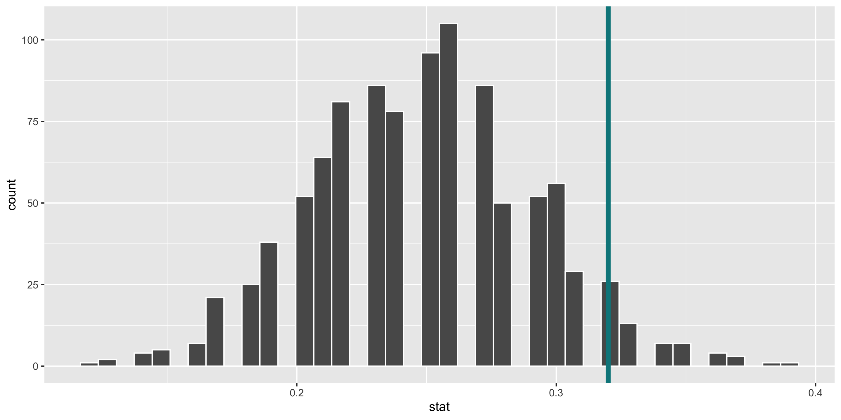
Computing Power
- Determine the “critical value(s)” where \(\alpha = 0.05\)
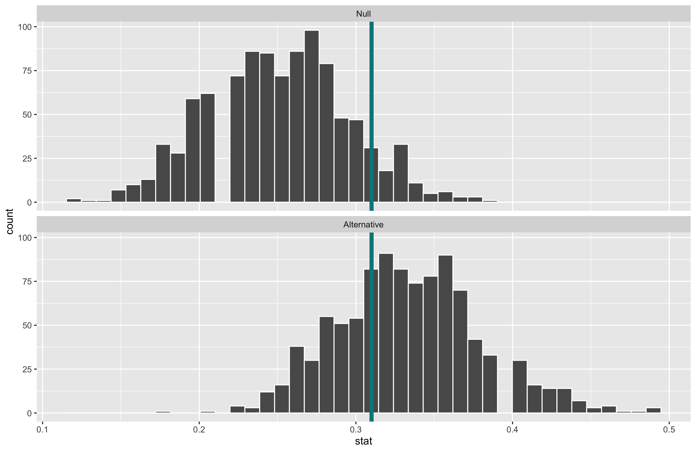
Computing Power
- Construct the alternative distribution.
alt <- dat %>%
  specify(response = at_bats, success = "hit") %>%
  hypothesize(null = "point", p = 0.333) %>%
  generate(reps = 1000, type = "draw") %>%
  calculate(stat = "prop")

ggplot(data = alt, mapping = aes(x = stat)) +
  geom_histogram(bins = 27, color = "white") +
  geom_vline(xintercept = quantile(null$stat, 0.95),
             size = 2,
             color = "turquoise4")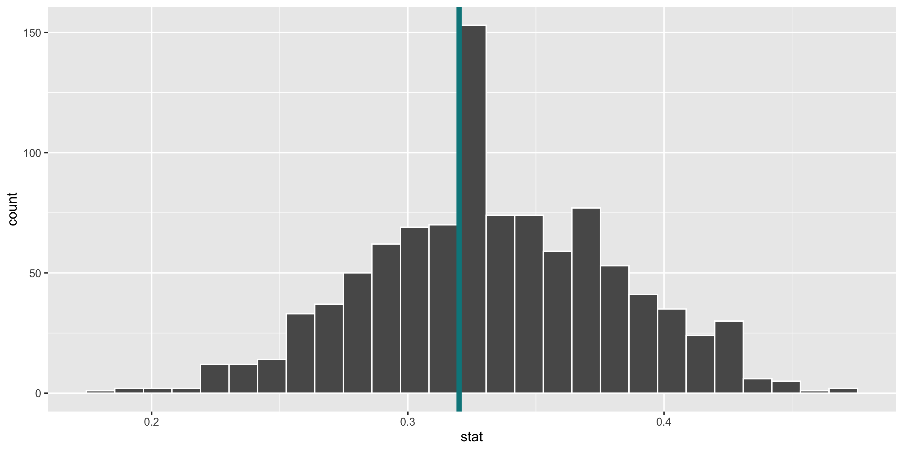
Reporting Results in Journal Articles
