
Random Variables III
Grayson White
Math 141
Week 10 | Fall 2025
Density Curve
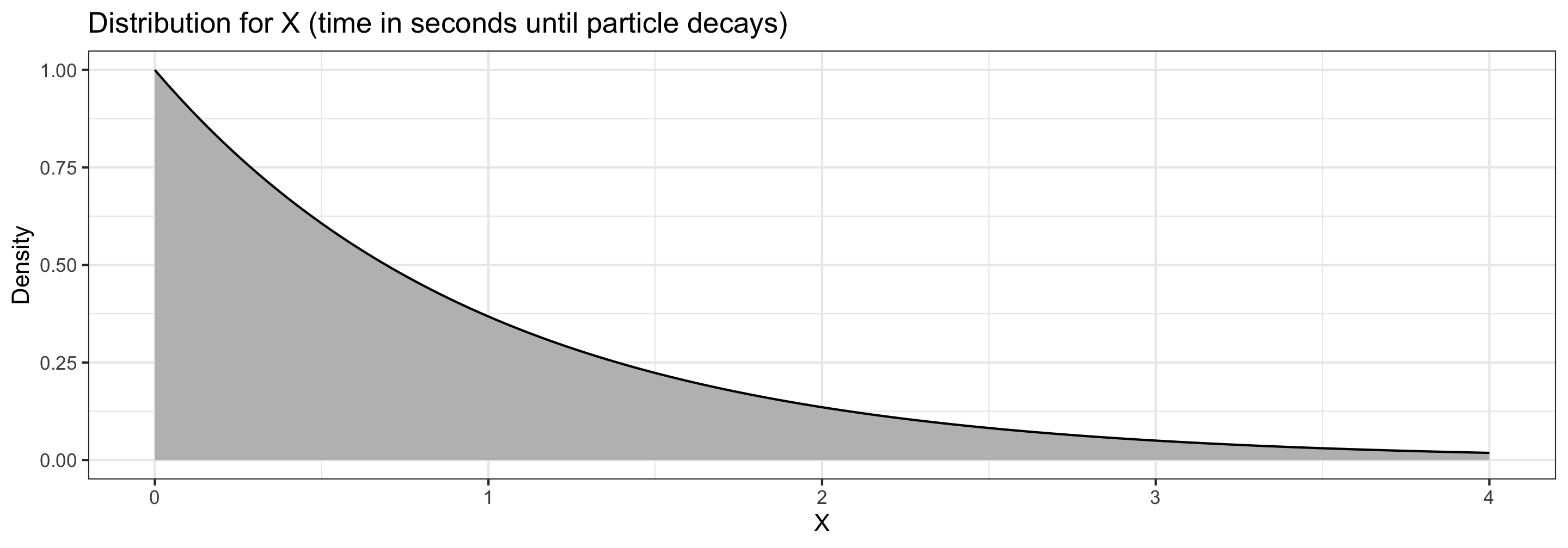
Suppose \(X\) is a random variable representing the time (in seconds) it takes for a particle to experience radioactive decay, where \[ f(x) = e^{-x} \qquad \textrm{for } x\geq 0 \]
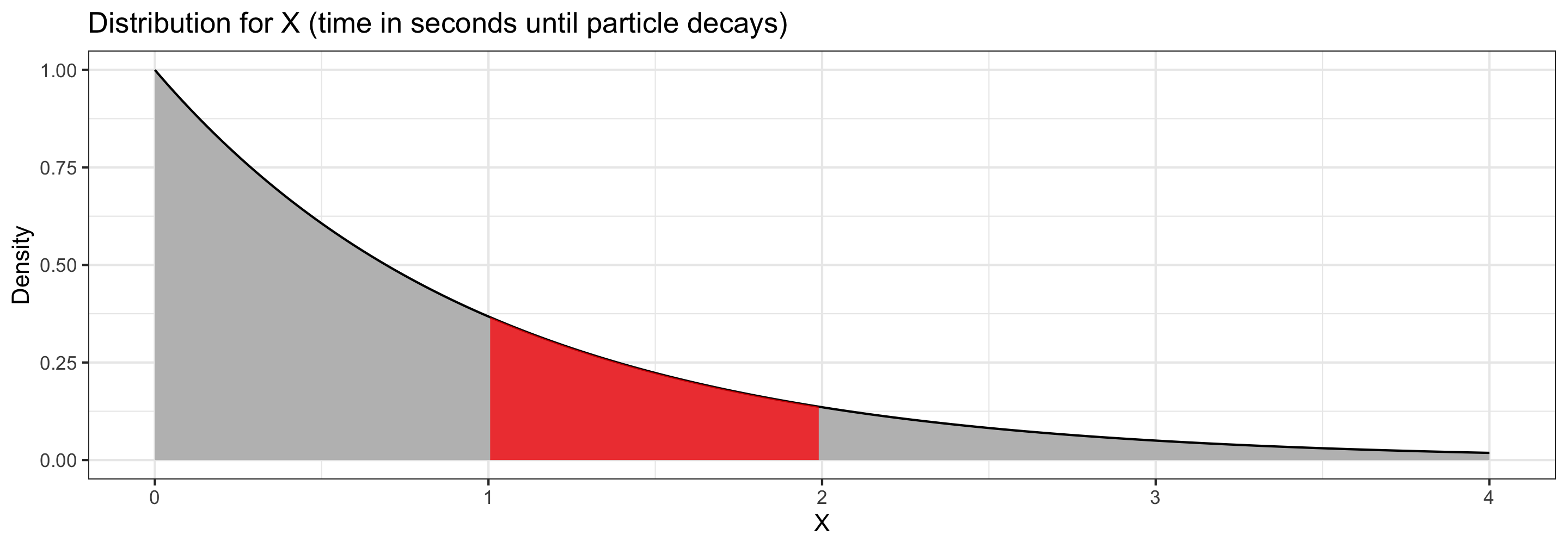
- The probability that it takes between \(1\) and \(2\) seconds to decay is the area under the curve between \(1\) and \(2\). \(P(1 < T < 2) = \color{red}{0.232}\)
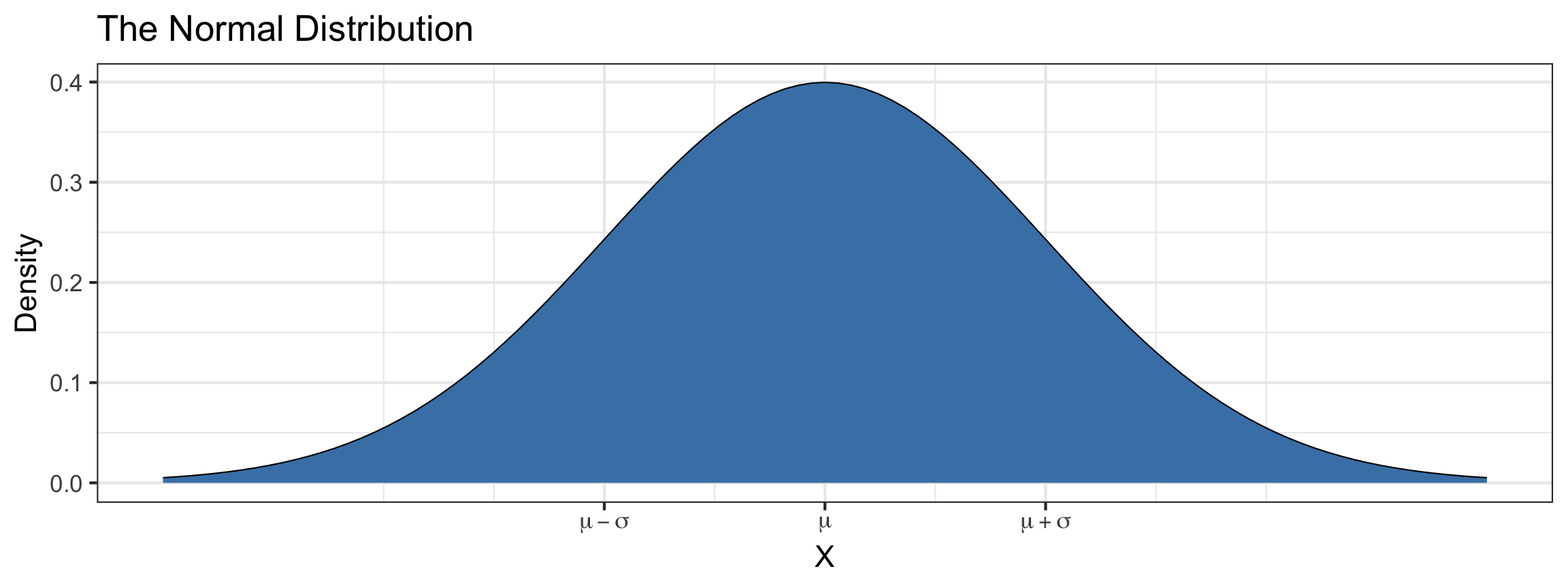
The Normal Distribution
The Normal distribution is defined by two parameters:
- Mean, \(\mu\)
- Standard deviation, \(\sigma\)
Suppose \(X\) follows a Normal(\(\mu\),\(\sigma\)) distribution. The density function is \[f(x) = \frac{1}{\sqrt{2 \pi \sigma^2}} \cdot\exp \left(\frac{-(x-\mu)^2}{2\sigma^2}\right)\]
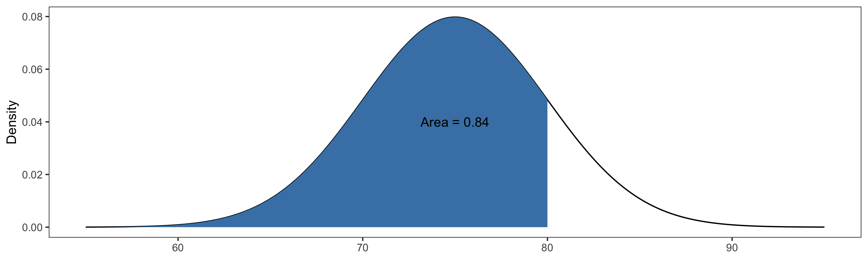
Calculating Probabilities
R has built-in functions for calculating probabilities from a normal distribution.
Suppose \(X\sim \text{Normal}(\mu=75, \sigma=5)\). Then:
Calculating Probabilities
R has built-in functions for calculating probabilities from a normal distribution.
Suppose \(X\sim \text{Normal}(\mu=75, \sigma=5)\). Then:
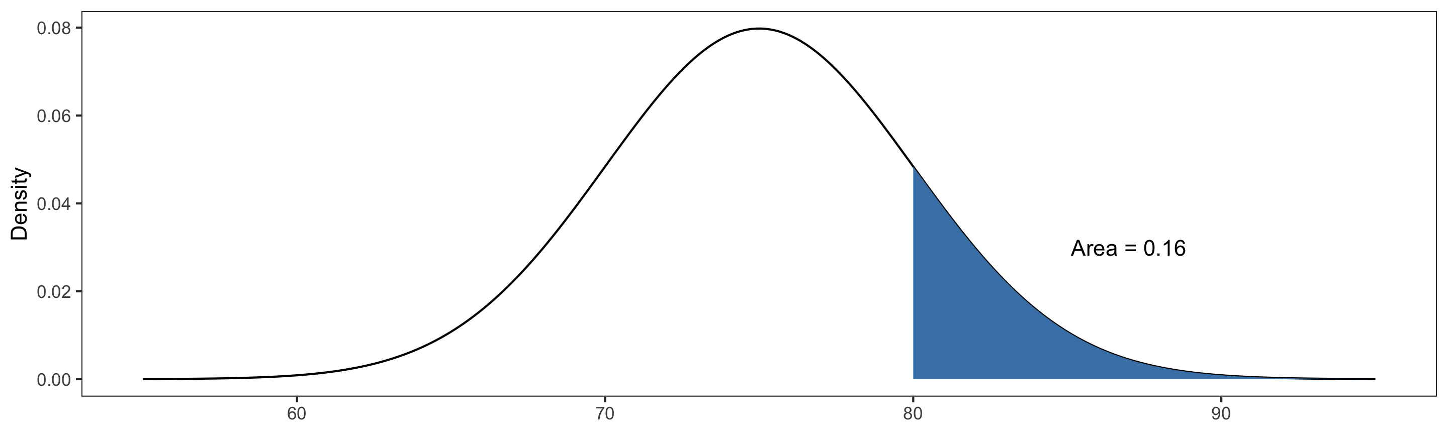
Calculating Probabilities
R has built-in functions for calculating probabilities from a normal distribution.
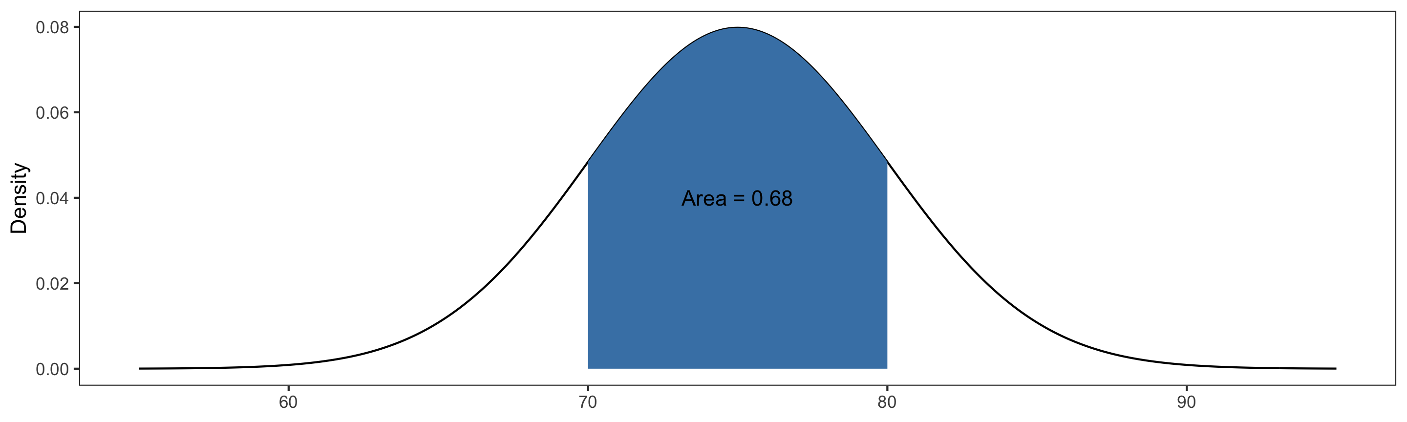
Suppose \(X\sim \text{Normal}(\mu=75, \sigma=5)\). Then:
- \(P(70 \leq X \leq 80) = P(X\leq 80) - P(X\leq 70) =\)
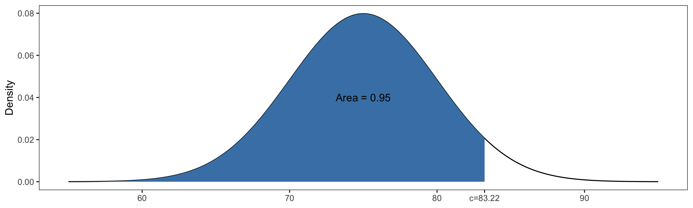
Finding Quantiles
We can also use R to find quantiles of a Normal distribution.
Suppose \(X\sim \text{Normal}(\mu=75, \sigma=5)\). Then:
Scale and Translation Invariance
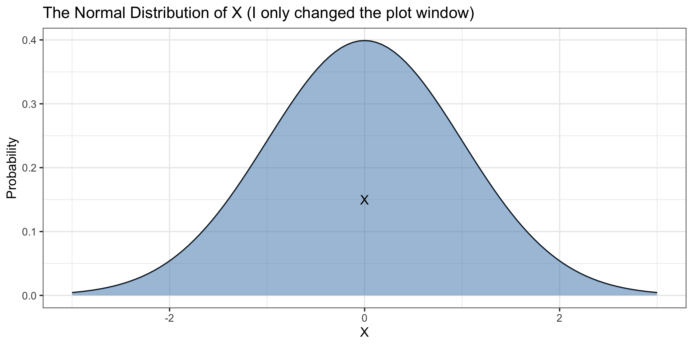
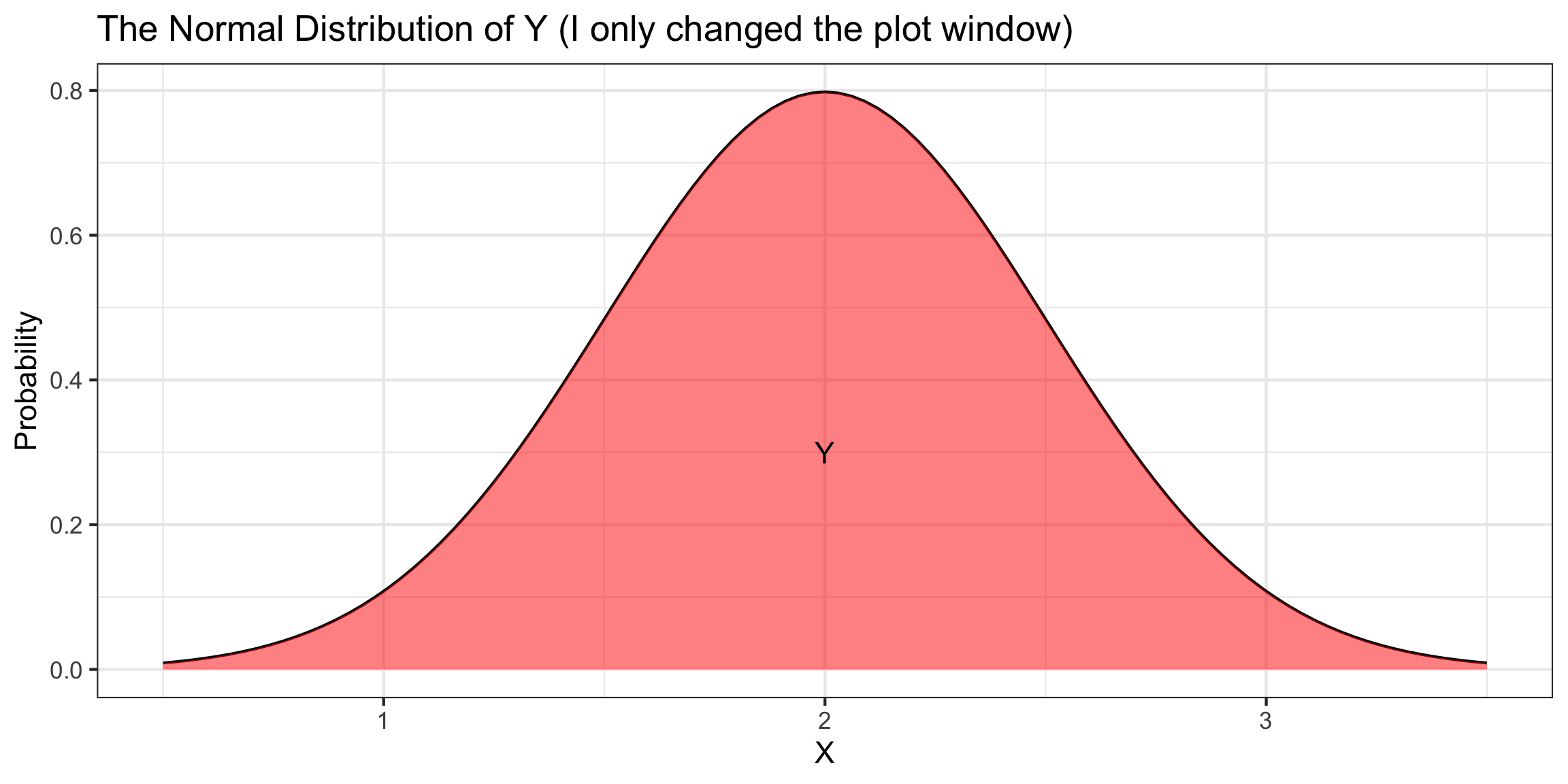
Suppose \(X\sim\text{Normal}(\mu=0,\sigma=1)\) and \(Y\sim\text{Normal}(\mu=2,\sigma=0.25)\).
\(X\) and \(Y\) have different means, heights, and widths…
- But the same shapes!
Scale and Translation Invariance
Suppose \(X\sim\text{Normal}(\mu=0,\sigma=1)\) and \(Y\sim\text{Normal}(\mu=2,\sigma=0.25)\).
\(X\) and \(Y\) have different means, heights, and widths…
- But the same shapes!
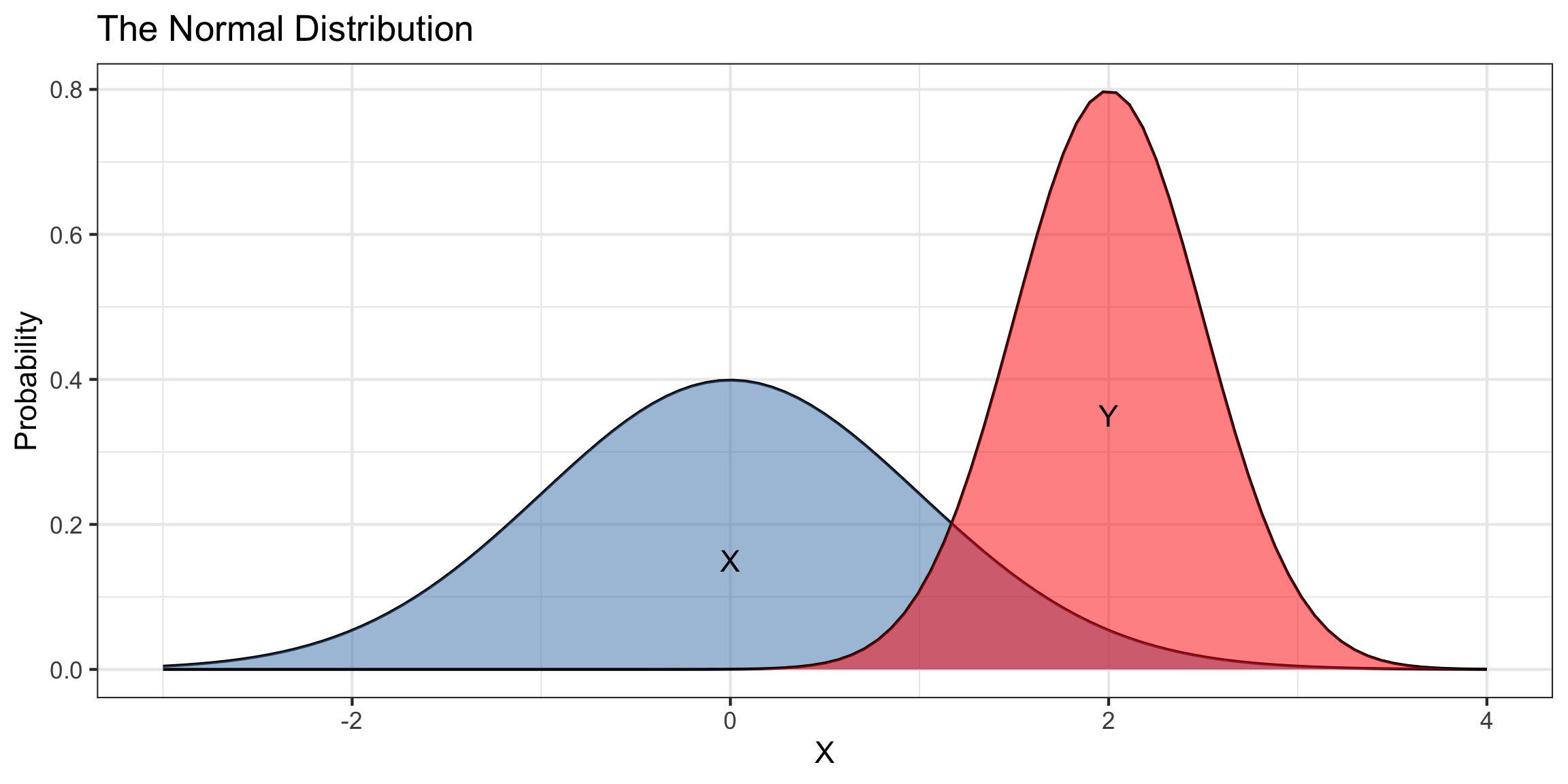
Scale and Translation Invariance
Suppose \(X\sim\text{Normal}(\mu=0,\sigma=1)\) and \(Y\sim\text{Normal}(\mu=2,\sigma=0.25)\).
\(X\) and \(Y\) have different means, heights, and widths…
- But the same shapes!
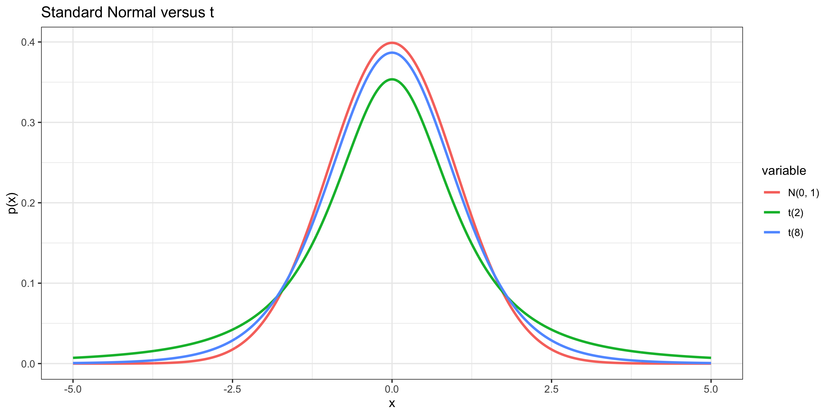
t distribution
\(X \sim\) t(df)
Distribution:
\[ f(x) = \frac{\Gamma(\mbox{df} + 1)}{\sqrt{\mbox{df}\pi} \Gamma(2^{-1}\mbox{df})}\left(1 + \frac{x^2}{\mbox{df}} \right)^{-\frac{df + 1}{2}} \]
where \(-\infty < x < \infty\)
Mean: 0
Standard deviation: \(\sqrt{\mbox{df}/(\mbox{df} - 2)}\)
Approximating These Distributions
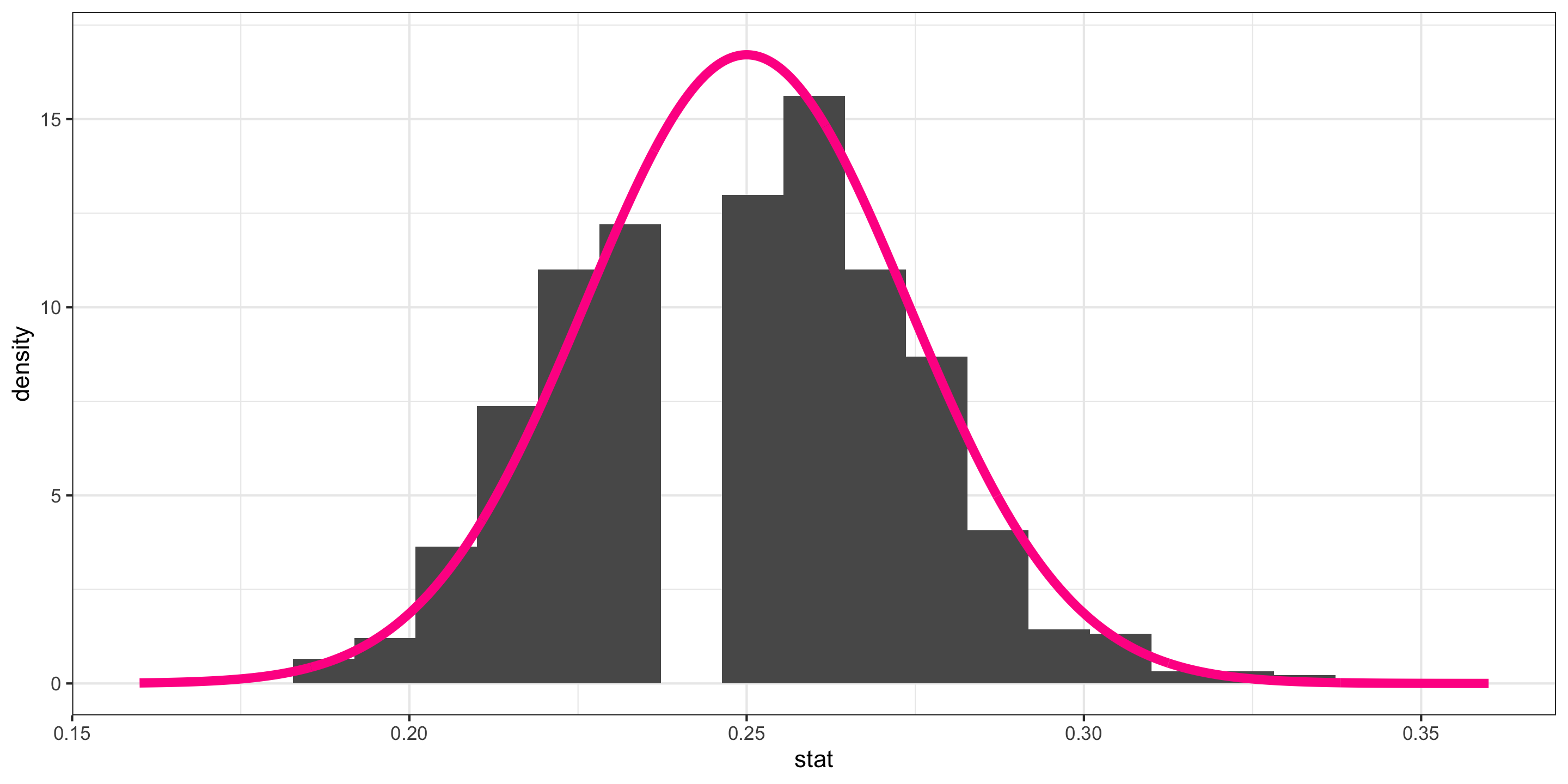
- \(\hat{p}\) = sample proportion of correct receiver guesses out of 329 ESP trials
We generated its Null Distribution:
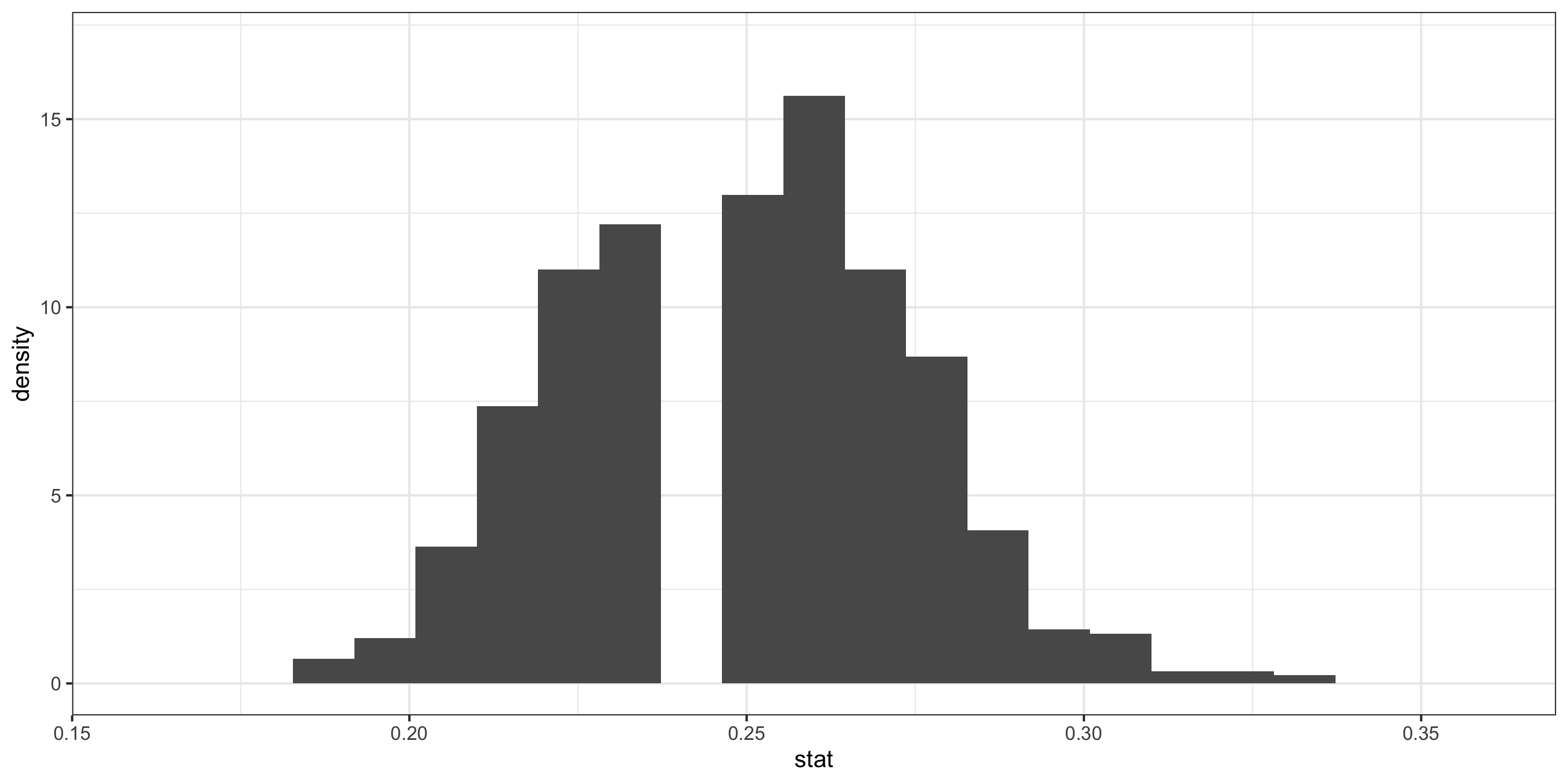
Which is well approximated by the distribution of a N(0.25, 0.024).
Approximating These Distributions
- \(\bar{x}_I - \bar{x}_N\) = difference in sample mean tuition between Ivies and non-Ivies
We generated its Null Distribution:
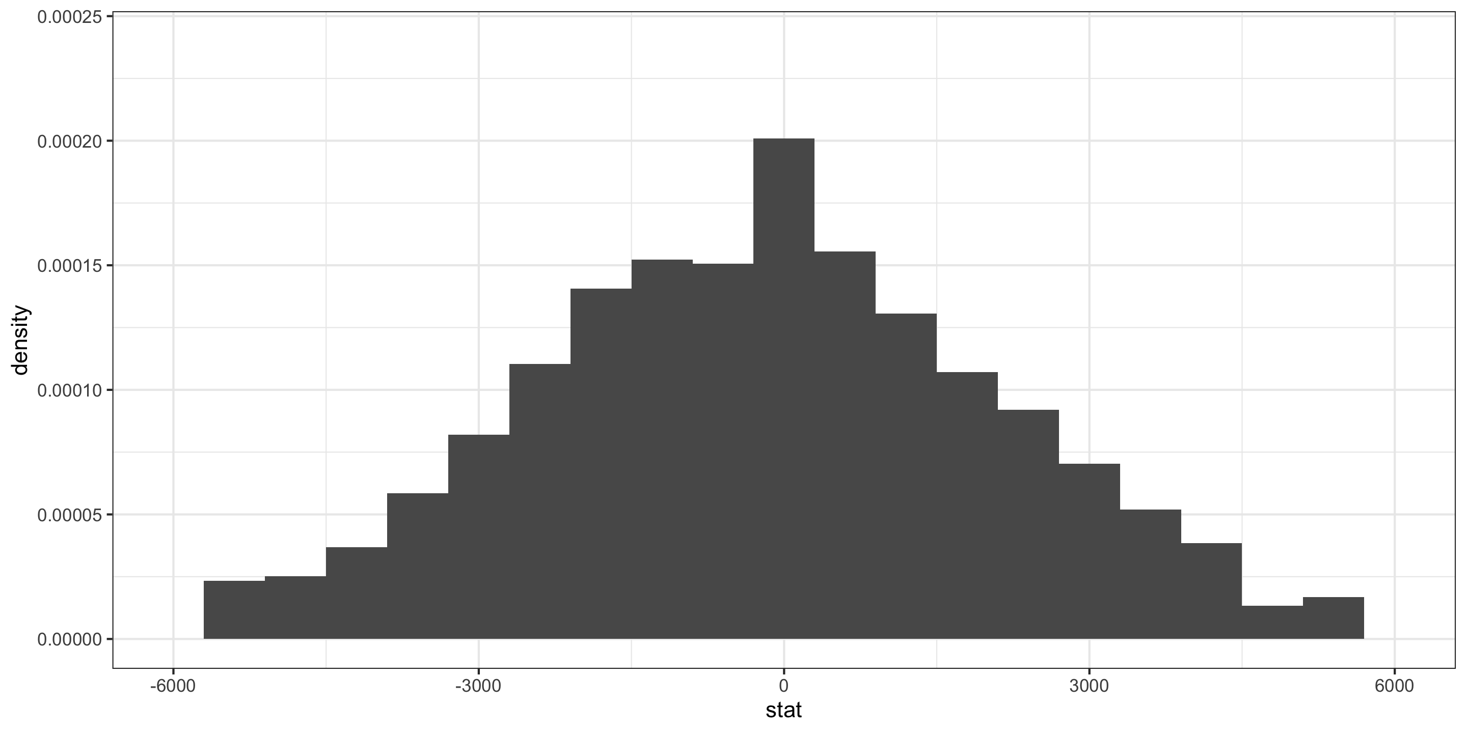
Which is somewhat approximated by the distribution of a N(0, 1036).
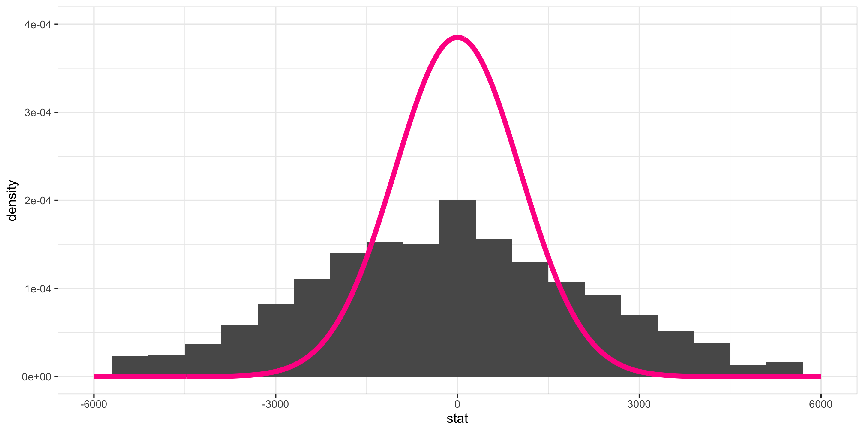
We will learn that a standardized version of the difference in sample means is better approximated by the distribution of a t(df = 7).
Approximating These Distributions
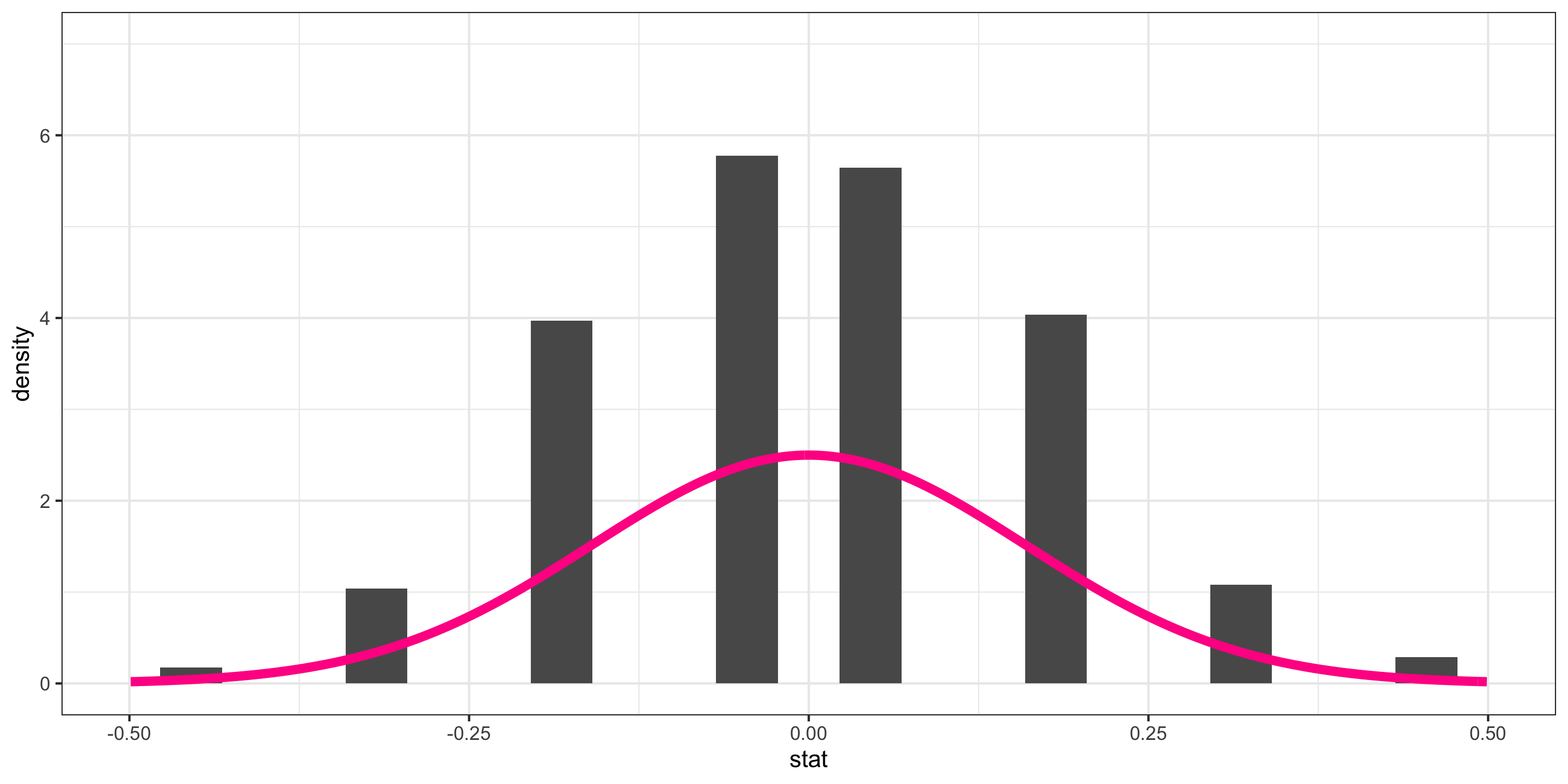
- \(\hat{p}_D - \hat{p}_Y\) = difference in sample improvement proportions between those who swam with dolphins and those who did not
We generated its Null Distribution:
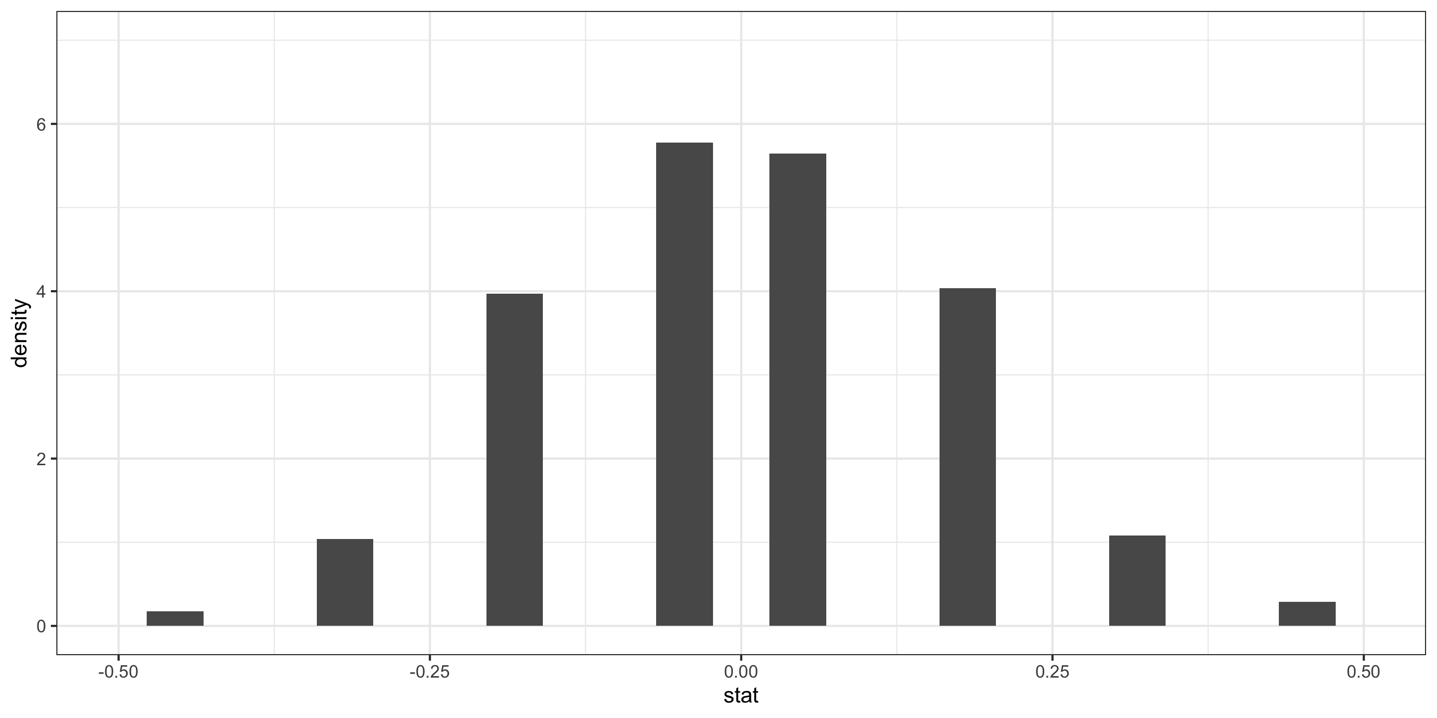
Which is kinda somewhat approximated by the probability function of a N(0, 0.16).
Approximating Sampling Distributions
Central Limit Theorem (CLT): For random samples and a large sample size \((n)\), the sampling distribution of many sample statistics is approximately normal.
Example: Japanese Flowering Cherry Trees at Portland’s Waterfront Park
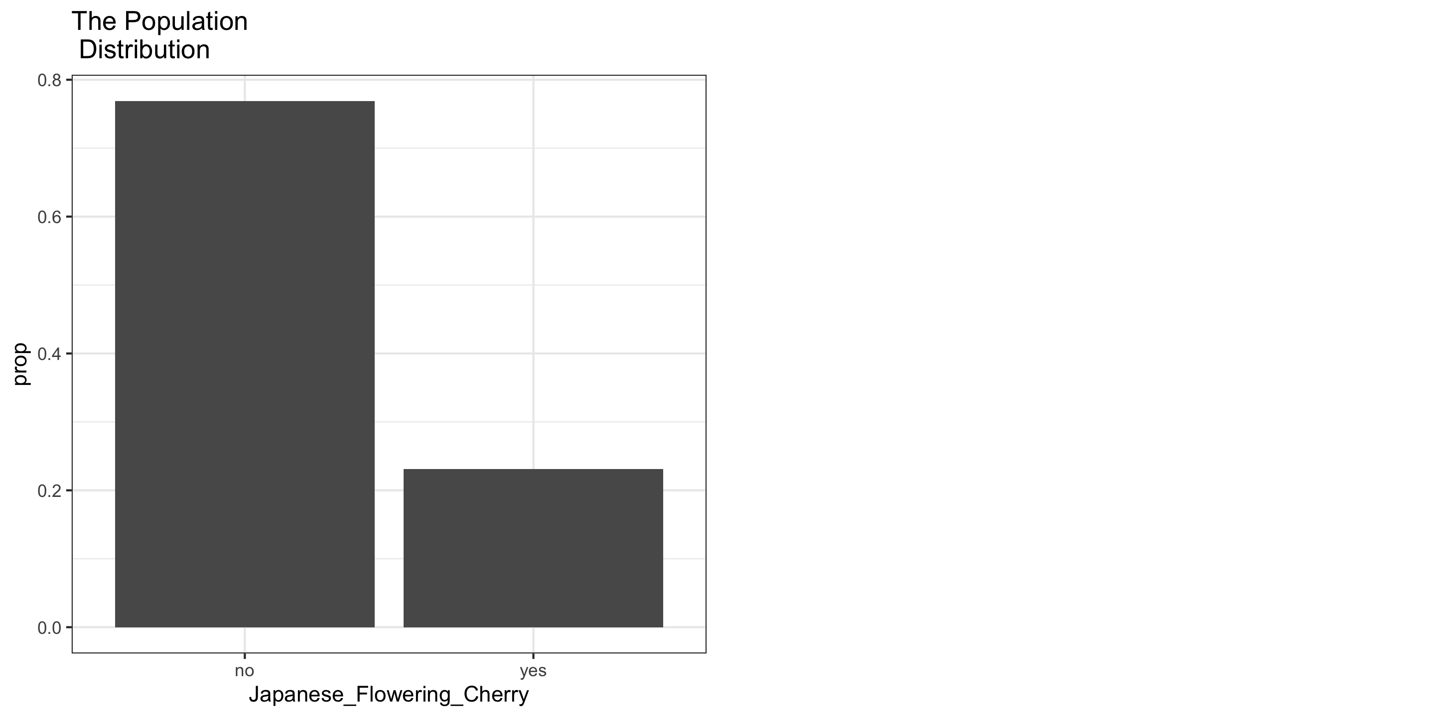
Approximating Sampling Distributions
Central Limit Theorem (CLT): For random samples and a large sample size \((n)\), the sampling distribution of many sample statistics is approximately normal.
Example: Japanese Flowering Cherry Trees at Portland’s Waterfront Park
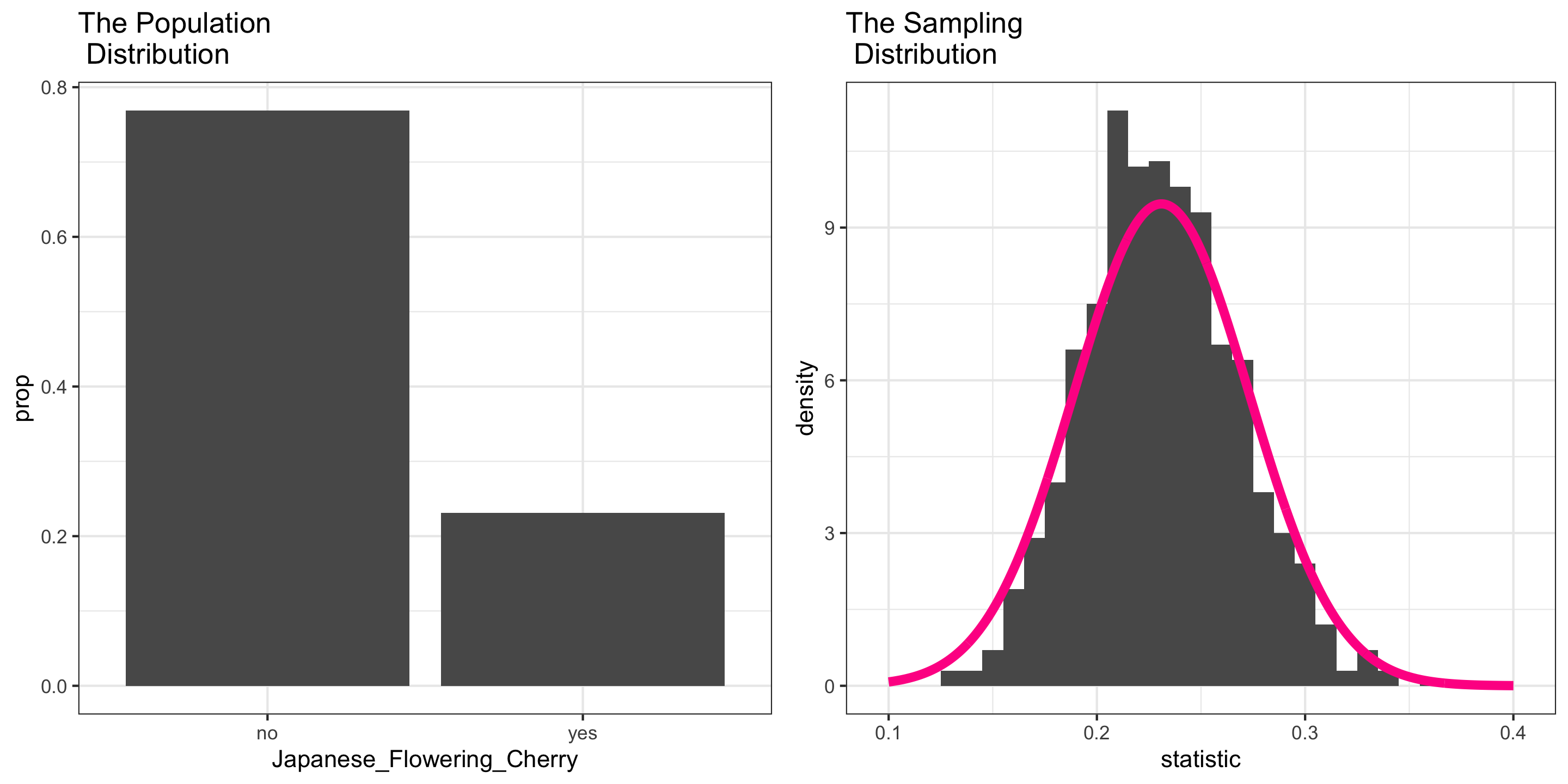
- But which Normal? (What is the value of \(\mu\) and \(\sigma\)?)