Today’s goal: introduction and recallation of linear regression
Next week: Deep dive + simulation based approach to inference for linear regression
But first: What class(es) should I take next in Statistics?
Available to you right after Math 141:
Math 241: Data Science
Offered this spring! A deep dive into all things data. Some topics we’ll think about next semester include: (interactive) data visualization, writing your own R packages, dashboarding, spatial data, ethics, text analysis, and much more!
No exams, no daily homework! Weekly lab assignments and a few projects through the semester.
Math 243: Statistical Learning
Offered next year. A deep dive into statistical modeling.
Applied courses further down the road:
Math 343: Practicum and Math 346: Bayesian Stats
Theory courses further down the road:
Math 391: Probability, Math 392: Mathematical Statistics, and Math 394: Causal Inference
Have Learned Two Routes to Statistical Inference
Which is better?
Is Simulation-Based Inference or Theory-Based Inference better?
Depends on how you define better.
If better = Leads to better understanding:
→ Research tends to show students have a better understanding of p-values and confidence from learning simulation-based methods.
If better = More flexible/robust to assumptions:
→ The simulation-based methods tend to be more flexible but that generally requires learning extensions beyond what we’ve seen in Math 141.
If better = More commonly used:
→ Definitely the theory-based methods but the simulation-based methods are becoming more common.
Good to be comfortable with both as you will find both approaches used in journal and news articles!
What does statistical inference (estimation and hypothesis testing) look like when I have more than 0 or 1 explanatory variables?
One route: Multiple Linear Regression!
Multiple Linear Regression
Linear regression is a flexible class of models that allow for:
Both quantitative and categorical explanatory variables.
Multiple explanatory variables.
Curved relationships between the response variable and the explanatory variable.
Should \(x_2\) be in the model that already contains \(x_1\) and \(x_3\)? Also often asked as “Controlling for \(x_1\) and \(x_3\), is there evidence that \(x_2\) has a relationship with \(y\)?”
After controlling for the other explanatory variables, what is the range of plausible values for \(\beta_3\) (which summarizes the relationship between \(y\) and \(x_3\))?
While \(\hat{y}\) is a point estimate for \(y\), can we also get an interval estimate for \(y\)? In other words, can we get a range of plausible predictions for \(y\)?
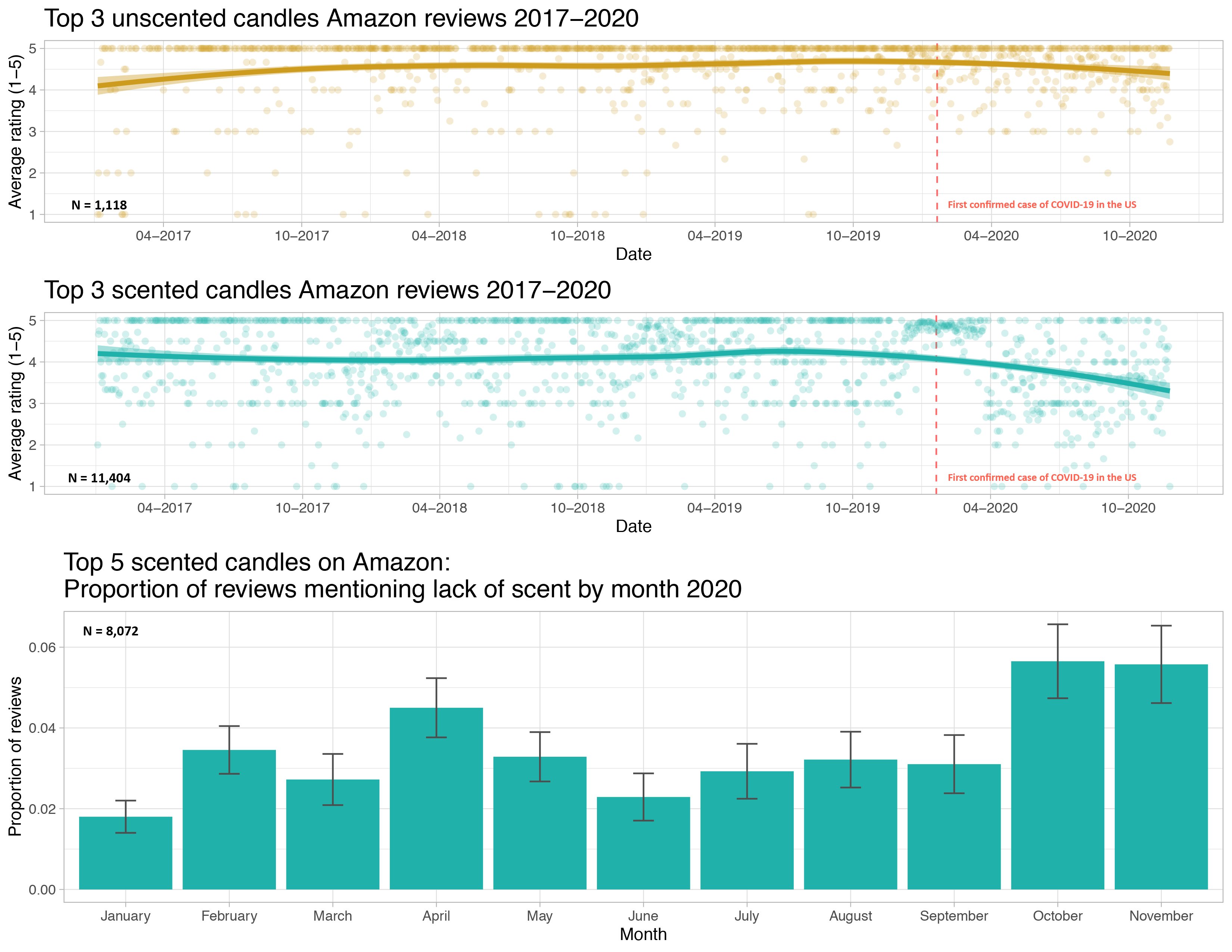
She posted all her data and code to GitHub and so we have the ability to play with it!
Do we have evidence that early in the pandemic the association between time and Amazon rating varies by whether or not a candle is scented and in particular, that scented candles have a steeper decline in ratings over time?
In other words, do we have evidence that we should allow the slopes to vary?
\[
H_o: \beta_j = 0 \quad \mbox{assuming all other predictors are in the model}
\]\[
H_a: \beta_j \neq 0 \quad \mbox{assuming all other predictors are in the model}
\]
Hypothesis Testing
Question: What tests is get_regression_table() conducting?
mod <-lm(Rating ~ Date + Type, data = all)get_regression_table(mod)
\[
H_o: \beta_2 = 0 \quad \mbox{given Date is already in the model}
\]\[
H_a: \beta_2 \neq 0 \quad \mbox{given Date is already in the model}
\]
Hypothesis Testing
Question: What tests is get_regression_table() conducting?
In General:
\[
H_o: \beta_j = 0 \quad \mbox{assuming all other predictors are in the model}
\]\[
H_a: \beta_j \neq 0 \quad \mbox{assuming all other predictors are in the model}
\]
Test Statistic: Let \(p\) = number of explanatory variables.
\[
t = \frac{\hat{\beta}_j - 0}{SE(\hat{\beta}_j)} \sim t(df = n - p)
\]
when \(H_o\) is true and the model assumptions are met.
There is evidence that including whether or not the candle is scented adds useful information to the linear regression model for Amazon ratings that already controls for date.
Example
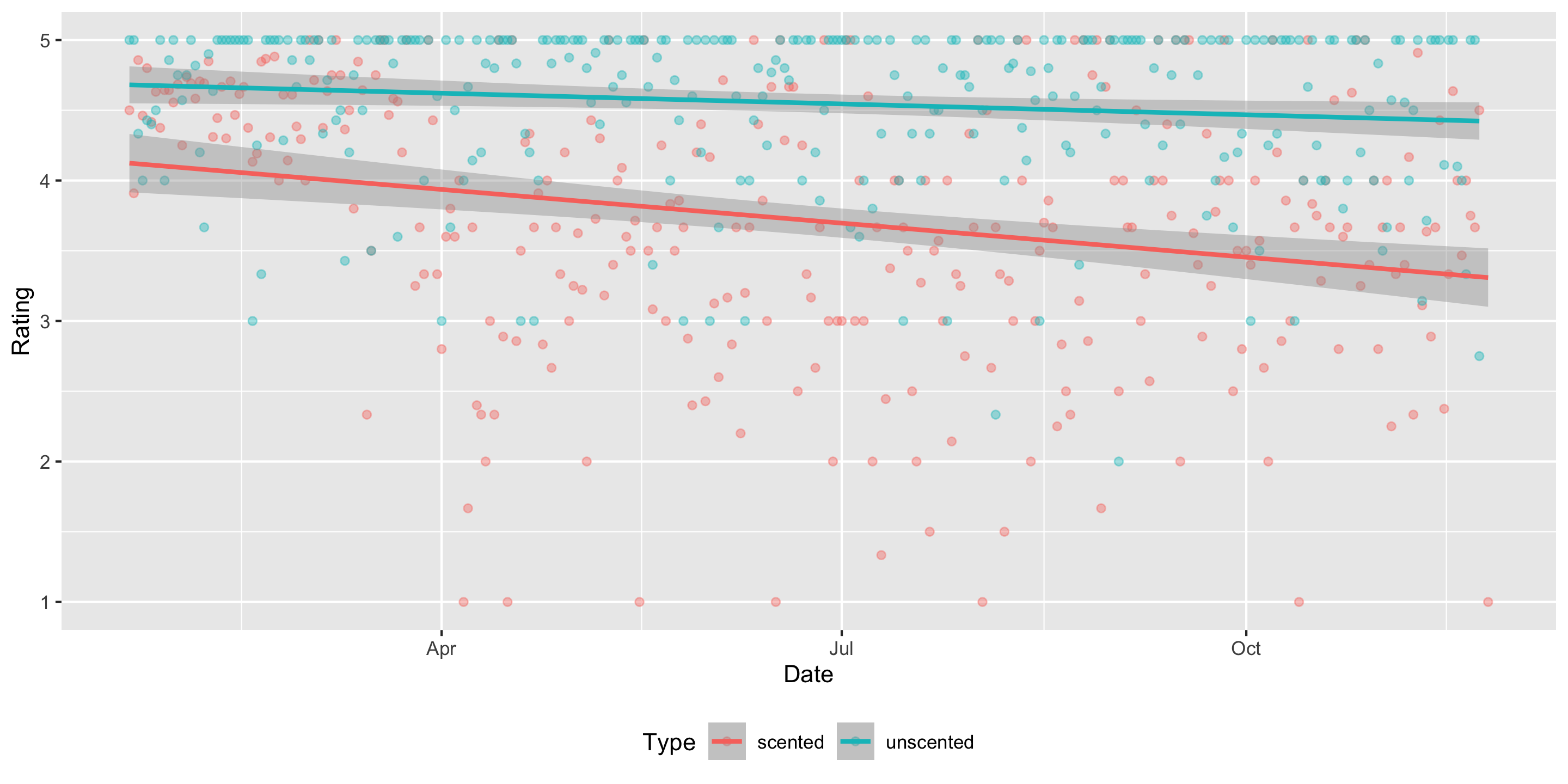
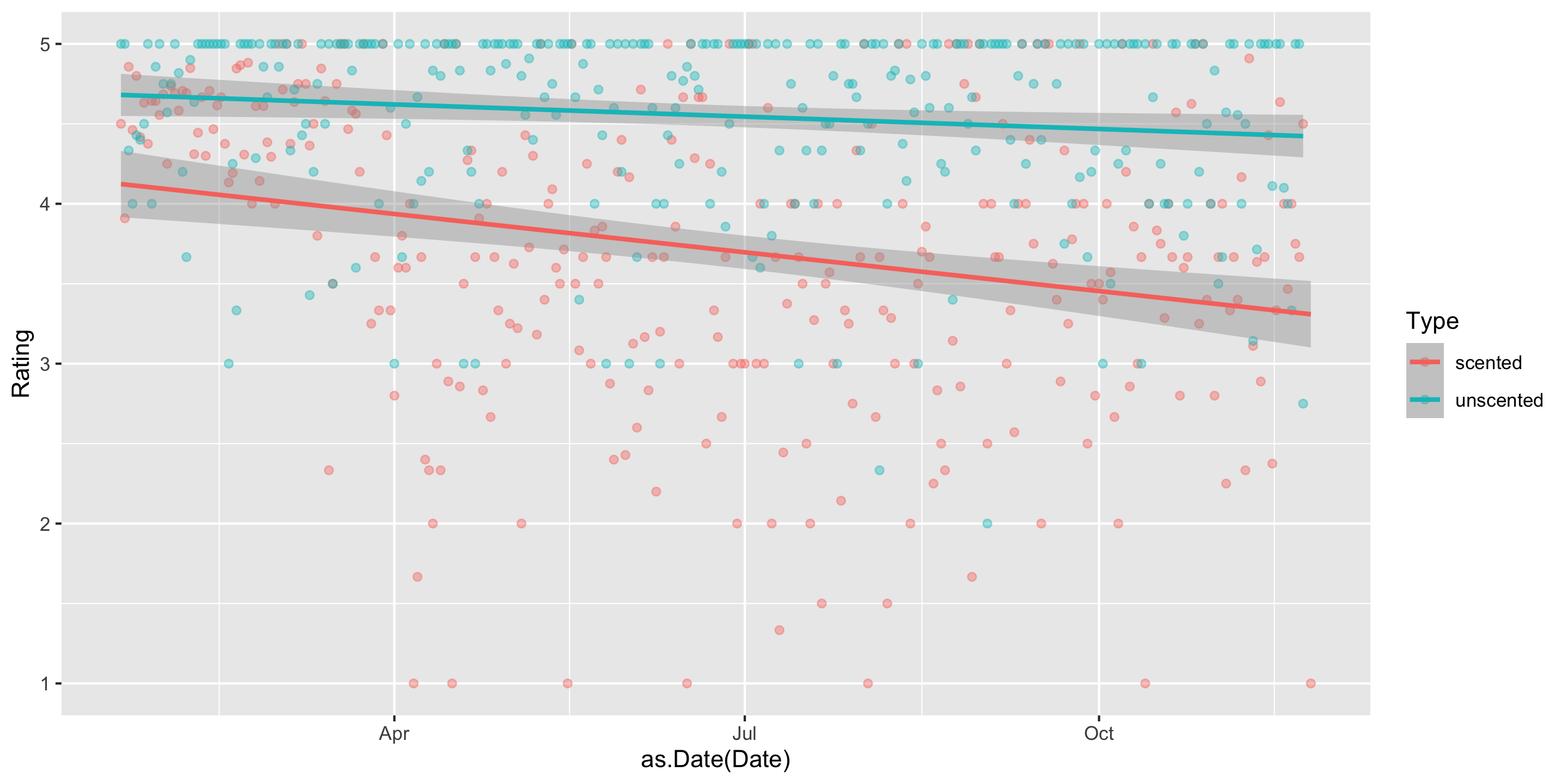
Do we have evidence that early in the pandemic the association between time and Amazon rating varies by whether or not a candle is scented and in particular, that scented candles have a steeper decline in ratings over time?
Do we have evidence that early in the pandemic the association between time and Amazon rating varies by whether or not a candle is scented and in particular, that scented candles have a steeper decline in ratings over time?
mod <-lm(Rating ~ Date * Type, data = all)get_regression_table(mod)
Now let’s shift our focus to estimation and prediction!
Estimation
Typical Inferential Question:
After controlling for the other explanatory variables, what is the range of plausible values for \(\beta_j\) (which summarizes the relationship between \(y\) and \(x_j\))?
While \(\hat{y}\) is a point estimate for \(y\), can we also get an interval estimate for \(y\)? In other words, can we get a range of plausible predictions for \(y\)?
Two Types of Predictions
Confidence Interval for the Mean Response
→ Defined at given values of the explanatory variables
→ Estimates the average response
→ Centered at \(\hat{y}\)
→ Smaller SE
Prediction Interval for an Individual Response
→ Defined at given values of the explanatory variables
→ Predicts the response of a single, new observation
→ Centered at \(\hat{y}\)
→ Larger SE
CI for mean response at a given level of X:
We want to construct a 95% CI for the average price of Saratoga Houses (in 2006!) where the houses meet the following conditions: 1500 square feet, 20 years old, 2 bathrooms, and have central air.
Interpretation: We are 95% confident that the average price of 20 year old, 1500 square feet Saratoga houses with central air and 2 bathrooms is between $199,919 and $211834.
PI for a new Y at a given level of X:
Say we want to construct a 95% PI for the price of an individual house that meets the following conditions: 1500 square feet, 20 years old, 2 bathrooms, and have central air.
Notice: Predicting for a new observation not the mean!
Interpretation: For a 20 year old, 1500 square feet Saratoga house with central air and 2 bathrooms, we predict, with 95% confidence, that the price will be between $73,885 and $337,869.