
CLT-based inference
Grayson White
Math 141
Week 11 | Fall 2025
Logistics
- Final exam format discussion.
Goals for Today
- Learn theory-based statistical inference methods.
- Learn about sample size calculations.
Introduce a new group of test statistics based on z-scores.
Generalize the SE method confidence interval formula.
Central Limit Theorem – Sampling Distributions
There is a version of the CLT for many of our sample statistics.
For Sample Proportion:
CLT: For large \(n\) (At least 10 successes and 10 failures),
\[ \hat{p} \sim N \left(p,~ \sqrt{\frac{p(1-p)}{n}} \right) \]
For Sample Mean:
CLT: For large \(n\) (At least 30 observations),
\[ \bar{x} \sim N \left(\mu,~ \frac{\sigma}{\sqrt{n}} \right) \]
- Power of the CLT: Provides formula for the SE!
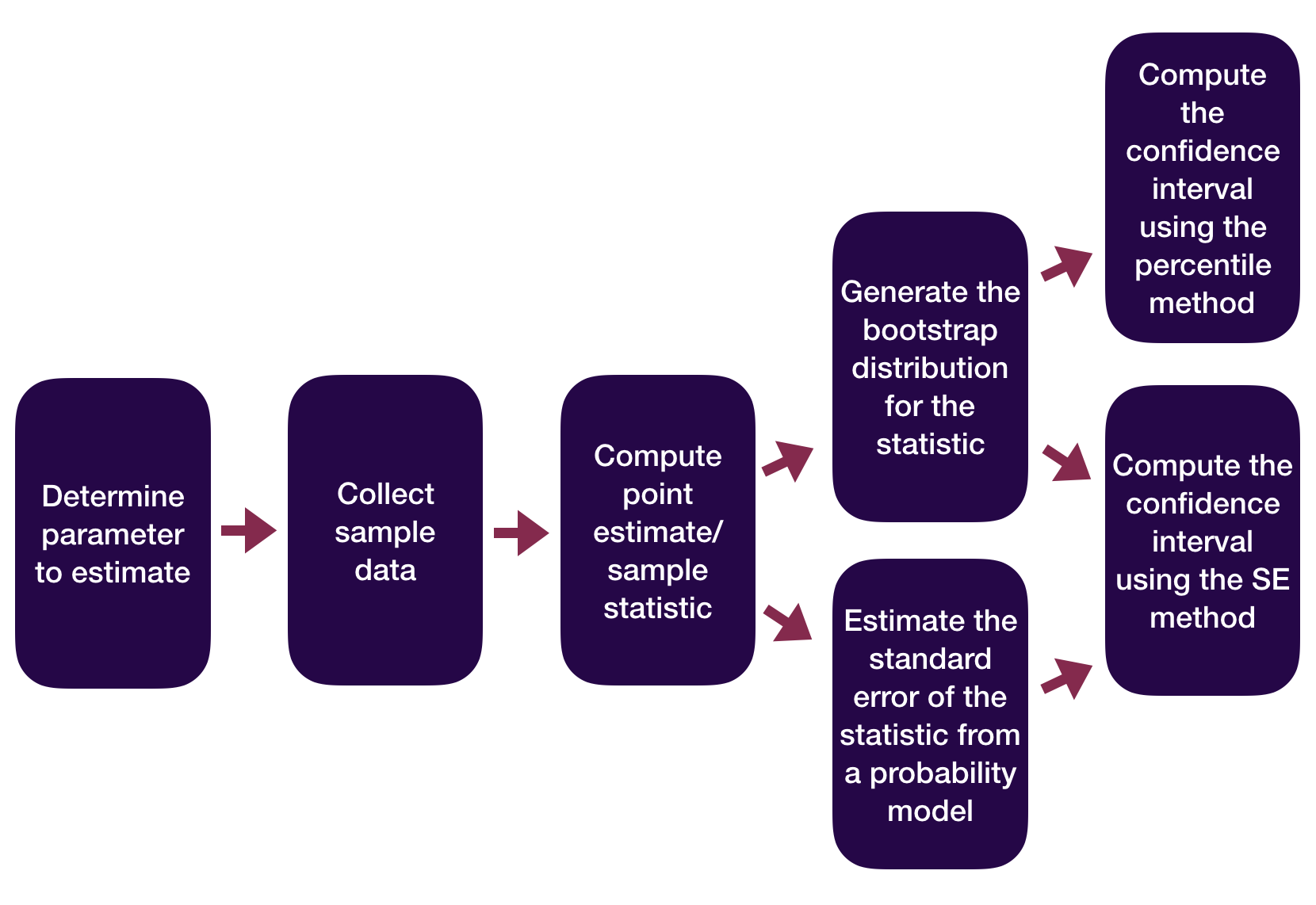
Statistical Inference Zoom Out – Estimation
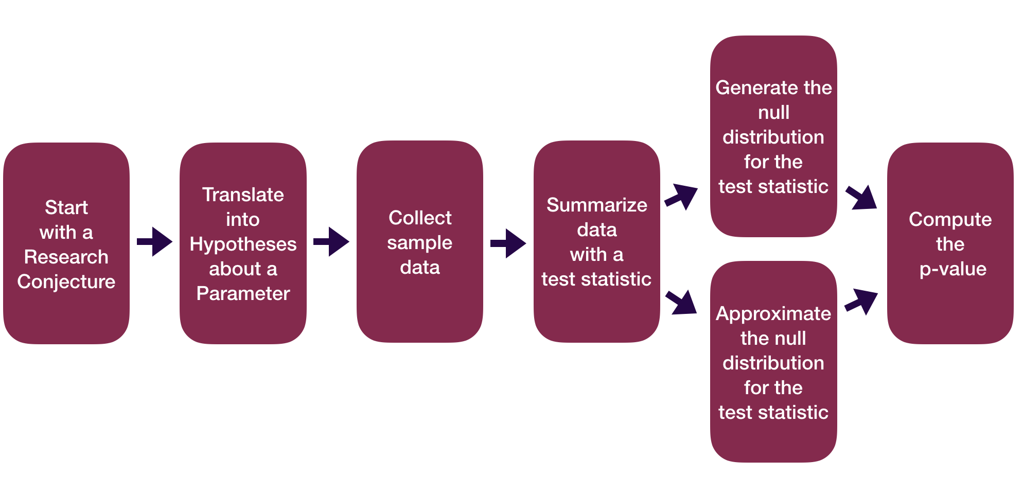
Statistical Inference Zoom Out – Testing
Sample Statistics as Random Variables
Sample statistics can be recast as random variables.
Need to figure out what random variable is a good approximation for our sample statistic.
- Then use the properties of that random variable to do inference.
Sometimes it is easier to find a good random variable approximation if we standardize our sample statistic first.
Z-scores
All of our test statistics so far have been sample statistics.
Another commonly used test statistic takes the form of a z-score:
\[ \mbox{Z-score} = \frac{X - \mu}{\sigma} \]
Standardized version of the sample statistic.
Z-score measures how many standard deviations the sample statistic is away from its mean.
Z-score Example

Z-score Example
- \(\hat{p}\) = proportion of Japanese Flowering Cherry trees in a sample of 100 trees
\[ \hat{p} \sim N \left(0.231, 0.042 \right) \]
- Suppose we have a sample where \(\hat{p} = 0.15\). Then the z-score would be:
\[ \mbox{Z-score} = \frac{0.15 - 0.231}{0.042} = -1.93 \]
Z-score Test Statistics
- A Z-score test statistic is one where we take our original sample statistic and convert it to a Z-score:
\[ \mbox{Z-score test statistic} = \frac{\mbox{statistic} - \mu}{\sigma} \]
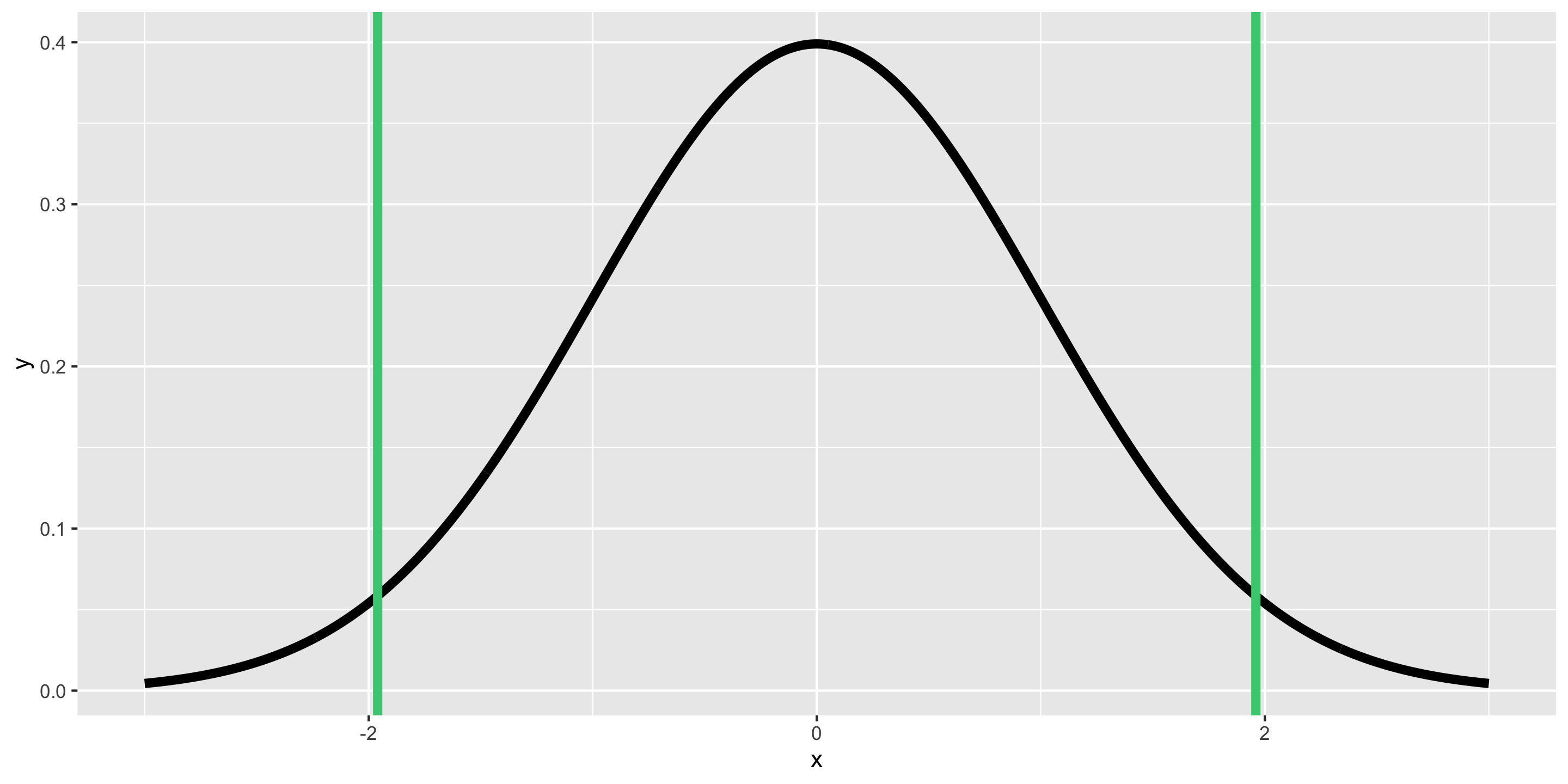
- Allows us to quickly (but roughly) classify results as unusual or not.
- \(|\) Z-score \(|\) > 2 → results are unusual/p-value will be smallish
- Commonly used because if the sample statistic \(\sim N(\mu, \sigma)\), then
\[ \mbox{Z-score test statistic} = \frac{\mbox{statistic} - \mu}{\sigma} \sim N(0, 1) \]
Let’s consider theory-based inference for a population proportion.
Inference for a Single Proportion – Testing
Let’s consider conducting a hypothesis test for a single proportion: \(p\)
Need:
- Hypotheses
- Same as with the simulation-based methods
- Test statistic and its null distribution
- Use a z-score test statistic and a standard normal distribution
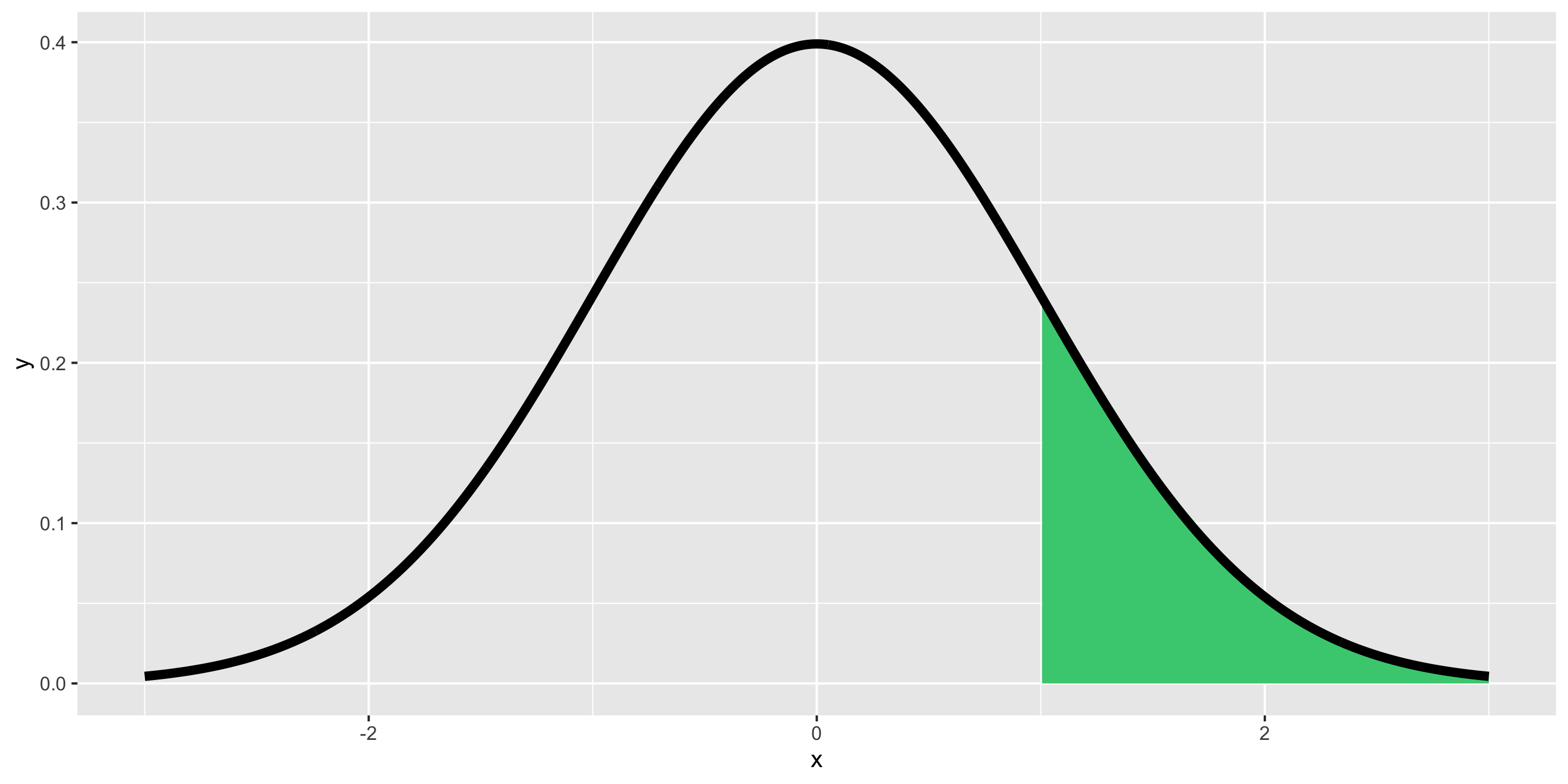
- P-value
- Compute from the standard normal distribution directly
Inference for a Single Proportion – Testing
Let’s consider conducting a hypothesis test for a single proportion: \(p\)
\(H_o: p = p_o\) where \(p_o\) = null value and \(H_a: p > p_o\) or \(H_a: p < p_o\) or \(H_a: p \neq p_o\)
By the CLT, under \(H_o\):
\[ \hat{p} \sim N \left(p_o, \sqrt{\frac{p_o(1-p_o)}{n}} \right) \]
Z-score test statistic:
\[ Z = \frac{\hat{p} - p_o}{\sqrt{\frac{p_o(1-p_o)}{n}}} \]
Use \(N(0, 1)\) to find the p-value once you have computed the test statistic.
Inference for a Single Proportion – Testing
Let’s consider conducting a hypothesis test for a single proportion: \(p\)
Example: Bern and Honorton’s (1994) extrasensory perception (ESP) studies
Inference for a Single Proportion – Testing
Let’s consider conducting a hypothesis test for a single proportion: \(p\)
Example: Bern and Honorton’s (1994) extrasensory perception (ESP) studies
Theory-Based Confidence Intervals
Suppose statistic \(\sim N(\mu = \mbox{parameter}, \sigma = SE)\).
95% CI for parameter:
\[ \mbox{statistic} \pm 1.96 SE \]
Theory-Based CIs in Action
Let’s consider constructing a confidence interval for a single proportion: \(p\)
By the CLT,
\[ \hat{p} \sim N \left(p,~ \sqrt{\frac{p(1-p)}{n}} \right) \]
P% CI for parameter:
\[\begin{align*} \mbox{statistic} \pm z^* SE \end{align*}\]Theory-Based CIs in Action
Example: Bern and Honorton’s (1994) extrasensory perception (ESP) studies
# Use probability model to approximate null distribution
prop_test(esp, response = guess, success = "correct",
          z = TRUE, conf_int = TRUE, conf_level = 0.95)
# A tibble: 1 × 5
statistic p_value alternative lower_ci upper_ci
<dbl> <dbl> <chr> <dbl> <dbl>
1 -6.45 1.12e-10 two.sided 0.274 0.374- Don’t use the reported test statistic and p-value!
Theory-Based CIs
P% CI for parameter:
\[ \mbox{statistic} \pm z^* SE \]
Notes:
Didn’t construct the bootstrap distribution.
Need to check that \(n\) is large and that the sample is random/representative.
- Condition depends on what parameter you are conducting inference for.
Interpretation of the CI doesn’t change.
For some parameters, the critical value comes from a \(t\) distribution.
Now we have a formula for the Margin of Error.
How do we perform probability model calculations in R?
Probability Calculations in R
Question: How do I compute probabilities in R?

Doesn’t seem quite right…
Probability Calculations in R
Question: How do I compute probabilities in R?
P*100% CI for parameter:
\[ \mbox{statistic} \pm z^* SE \]
P*100% CI for parameter:
\[ \mbox{statistic} \pm z^* SE \]
Probability Calculations in R
To help you remember:
Want a Probability?
→ use pnorm(), pt(), …
Want a Quantile (i.e. percentile)?
→ use qnorm(), qt(), …
Probability Calculations in R
Question: When might I want to do probability calculations in R?
Computed a test statistic that is approximated by a named random variable. Want to compute the p-value with
p---()Compute a confidence interval. Want to find the critical value with
q---().To do a Sample Size Calculation.
Sample Size Calculations
Very important part of the data analysis process!
Happens BEFORE you collect data.
You determine how large your sample size needs for a desired precision in your CI.
- The power calculations from hypothesis testing relate to this idea.
Sample Size Calculations
Question: Why do we need sample size calculations?
Example: Let’s return to the dolphins for treating depression example.
With a sample size of 30 and 95% confidence, we estimate that the improvement rate for depression is between 14.5 percentage points and 75 percentage points higher if you swim with a dolphin instead of swimming without a dolphin.
With a width of 60.5 percentage points, this 95% CI is a wide/very imprecise interval.
Question: How could we make it narrower? How could we decrease the Margin of Error (ME)?
Sample Size Calculations – Single Proportion
Let’s focus on estimating a single proportion. Suppose we want to estimate the current proportion of Reedies with COVID with 95% confidence and we want the margin of error on our interval to be less than or equal to 0.02. How large does our sample size need to be?
Want
\[ z^* \sqrt{\frac{\hat{p}(1 - \hat{p})}{n}} \leq B \]
Need to derive a formula that looks like
\[ n \geq \quad ... \]
Question: How can we isolate \(n\) to be on a side by itself?
Sample Size Calculations – Single Proportion
Let’s focus on estimating a single proportion. Suppose we want to estimate the current proportion of Reedies with COVID with 95% confidence and we want the margin of error on our interval to be less than or equal to 0.02. How large does our sample size need to be?
Sample size calculation:
\[ n \geq \frac{\hat{p}(1 - \hat{p})z^{*2}}{B^2} \]
What do we plug in for, \(\hat{p}\), \(z^{*}\), \(B\)?
Consider sample size calculations when estimating a mean on this week’s lab!
Statistical Inference using Probability Models
We went through theory-based inference for \(p\).
There are similar results for other parameters. But the specific named random variable may change!
- Will extend beyond inference for \(p\) next time.