CLT-based inference
Grayson White
Math 141
Week 11 | Fall 2025
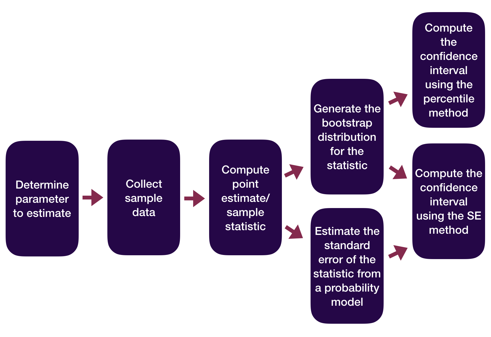
Statistical Inference Zoom Out – Estimation
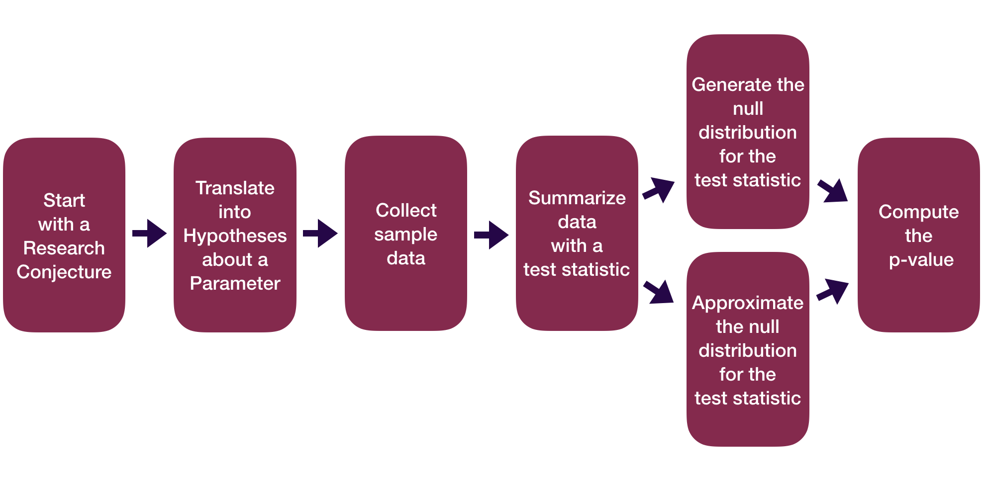
Statistical Inference Zoom Out – Testing
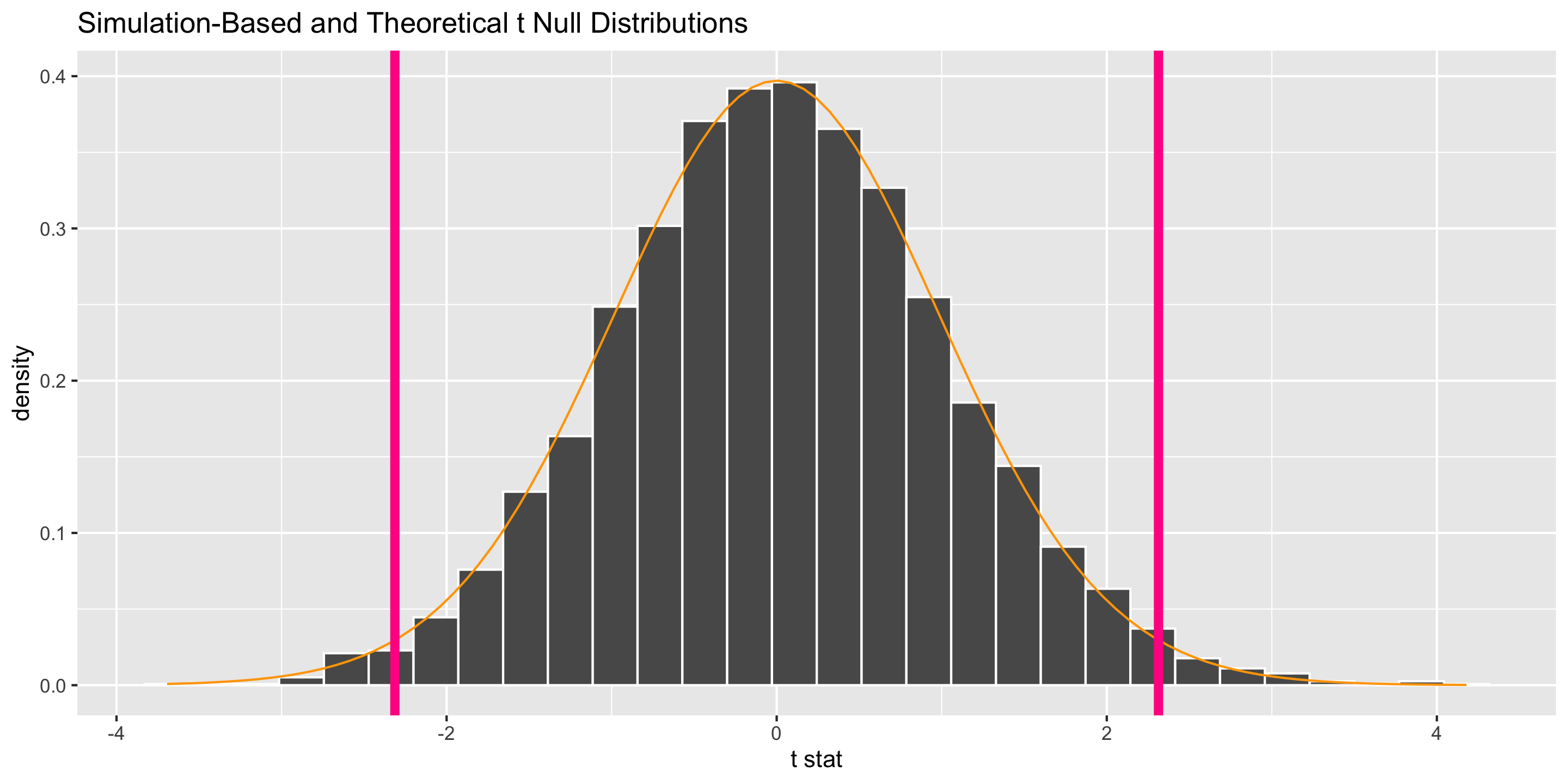
Inference for a Single Mean
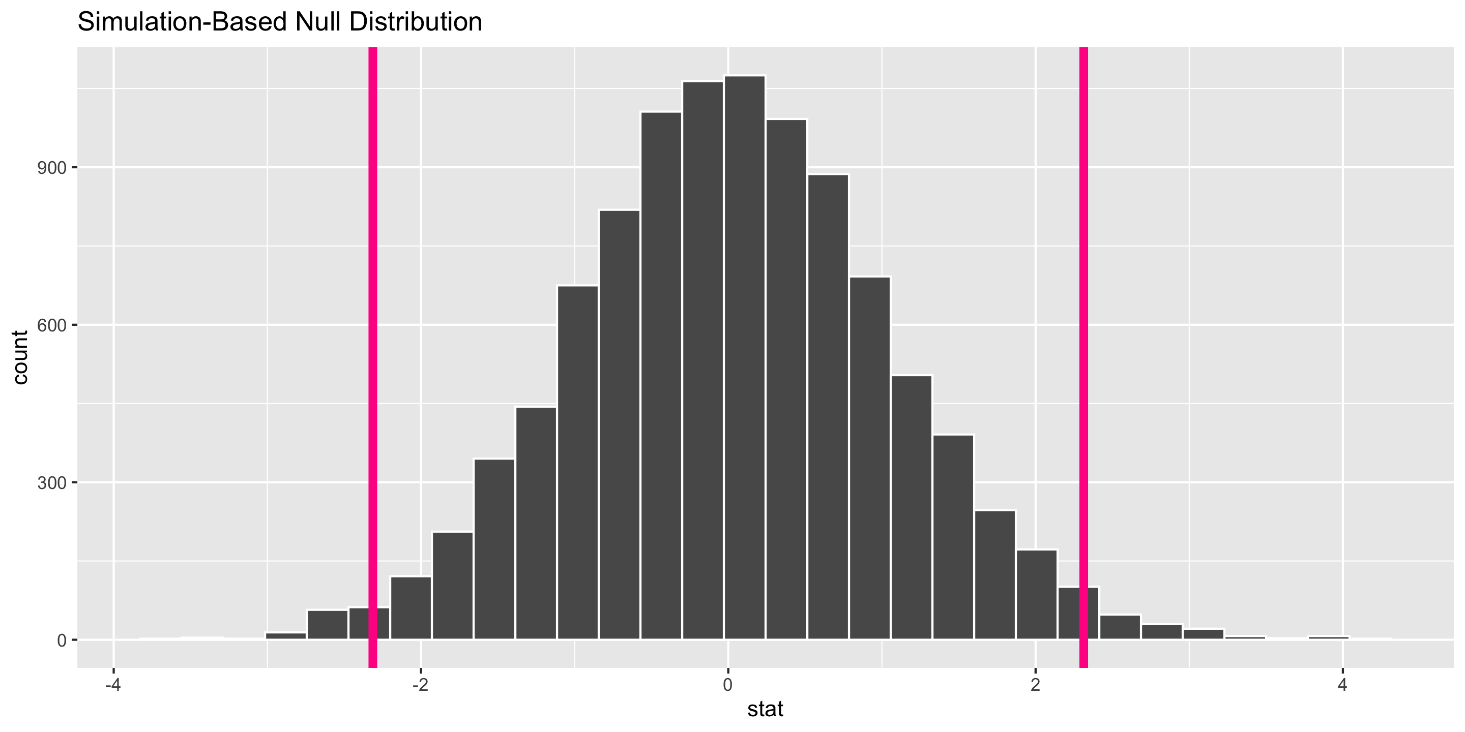
What probability function is a good approximation to the null distribution?
Inference for a Single Mean
What probability function is a good approximation to the null distribution?
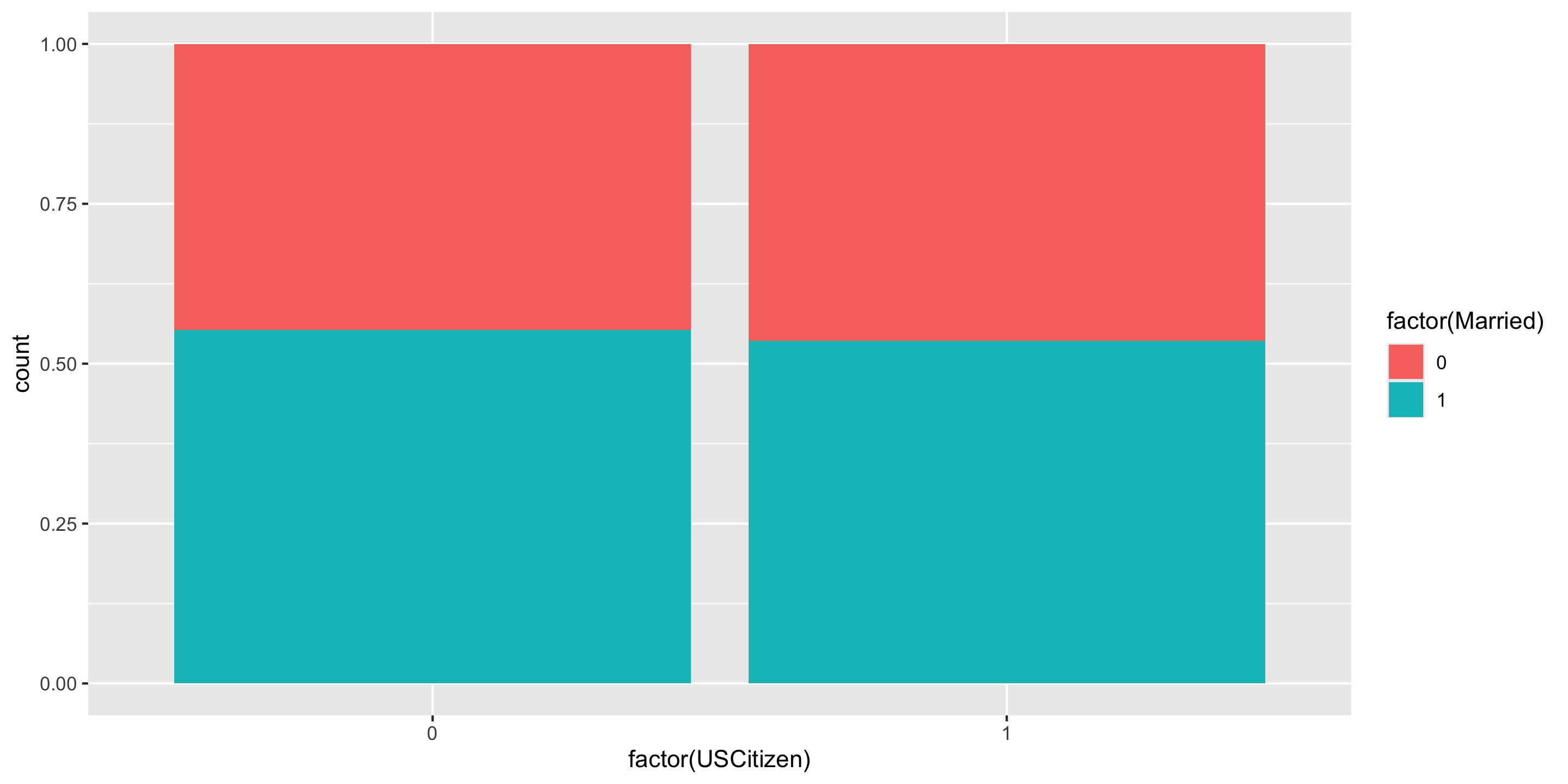
Difference in Proportions
Let’s try to determine if there’s a relationship between US citizenship and marriage status.
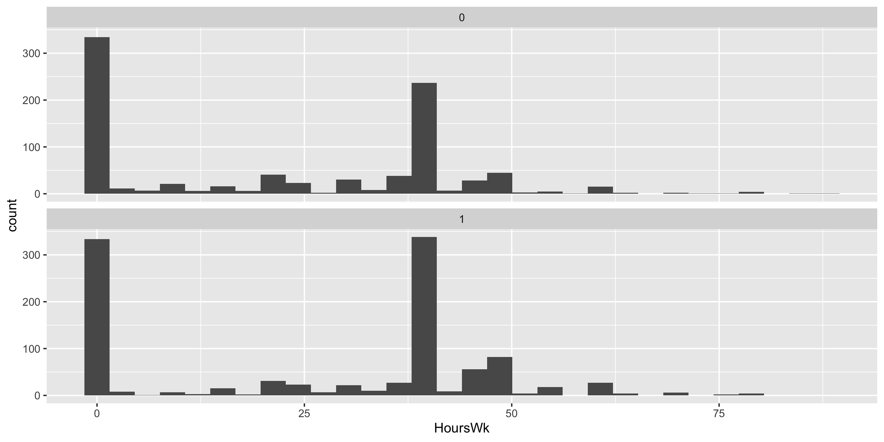
Difference in Means
Let’s estimate the average hours worked per week between married and unmarried US residents.
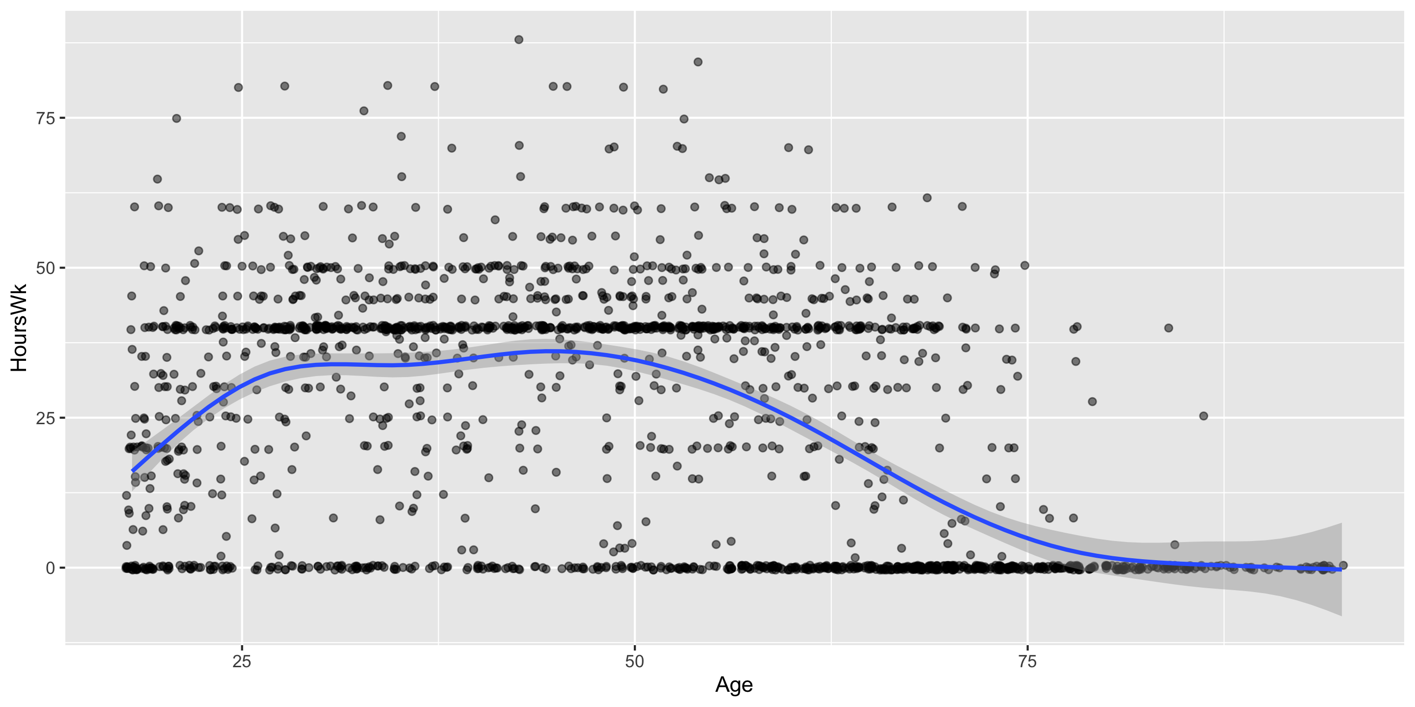
Correlation
We want to determine if age and hours worked per week have a positive linear relationship.
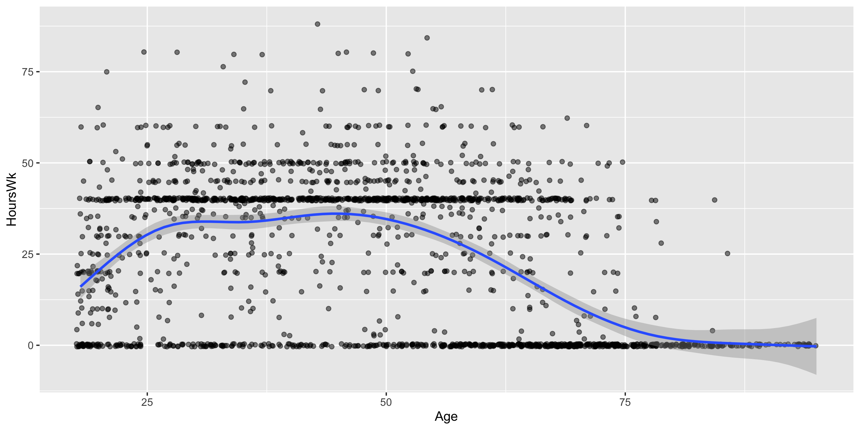
Correlation
We want to determine if age and hours worked per week have a positive linear relationship.