# A tibble: 6 × 11
  CN      county canopy_cover  elev   ppt tmean tmin01   tri   def   tnt biomass
  <chr>   <chr>         <int> <int> <int> <int>  <int> <dbl> <int> <int>   <dbl>
1 402196… 41001            24  1399   526   630   -847  13.1   585     1   6.11
2 345934… 41001            22  1329   430   745   -652  28.1   640     1   0.468
3 558628… 41001             7  1496   482   756   -648  15     654     2   1.42
4 484818… 41001            49  1836   856   451   -848  17.8   397     1   6.92
5 445418… 41001            46  1569   658   526  -1023  13.6   557     1   6.57
6 558628… 41001 48 1381 546 668 -666 16 518 1 2.59 
Regression Inference II
Grayson White
Math 141
Week 12 | Fall 2025
Example for Today: Forest Service data in Oregon
Today, we’ll use data from the US Forest Service, Forest Inventory & Analysis Program.


- The FIA program collects forest plot data on forest attributes across the United States.
- They also rely on remotely sensed data to model relationships between forest variables and remotely sensed variables.
- Each row in our dataset represents a plot. We include a forest variable (biomass) and remotely sensed predictors.
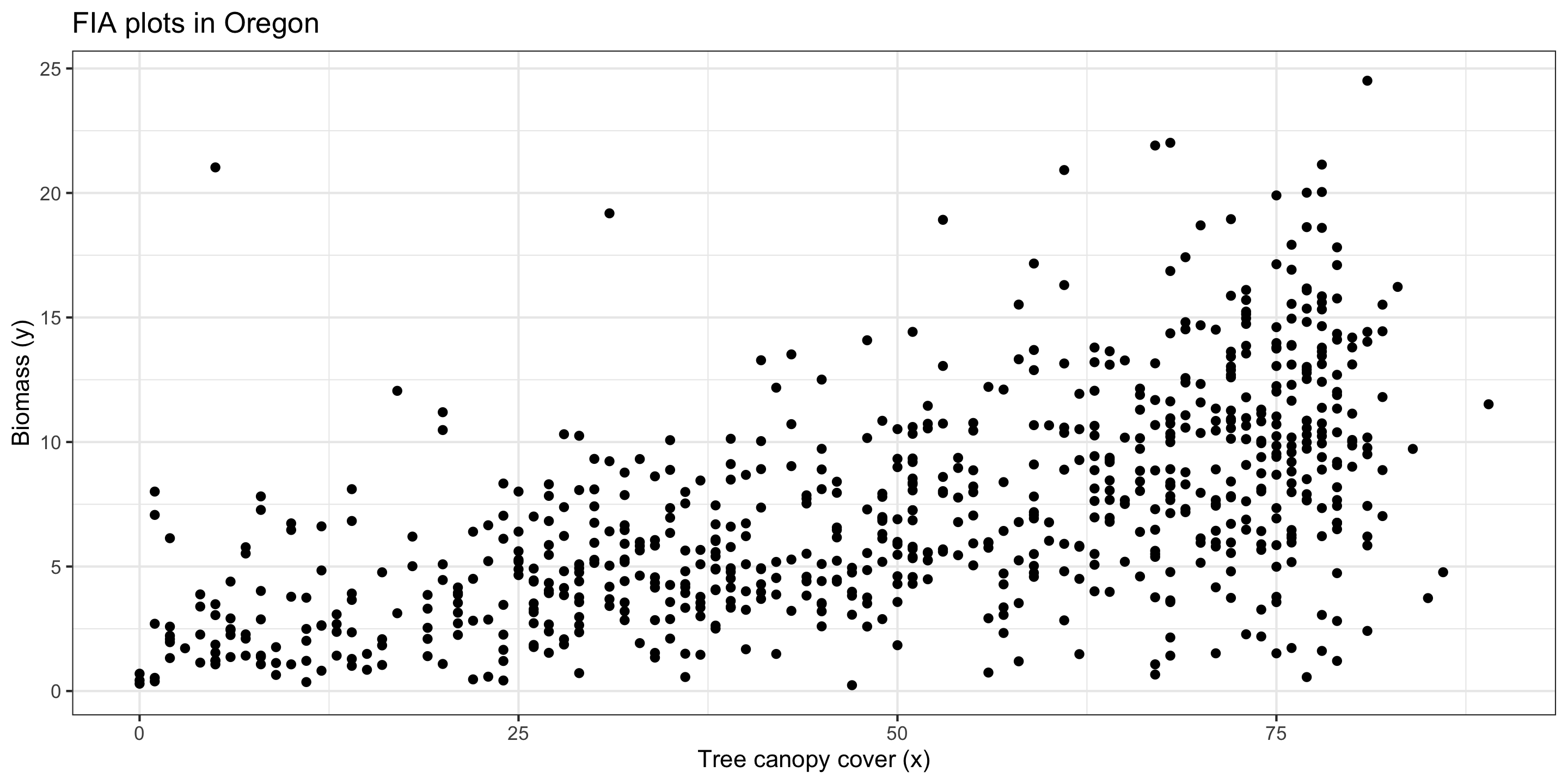
Oregon biomass data: EDA
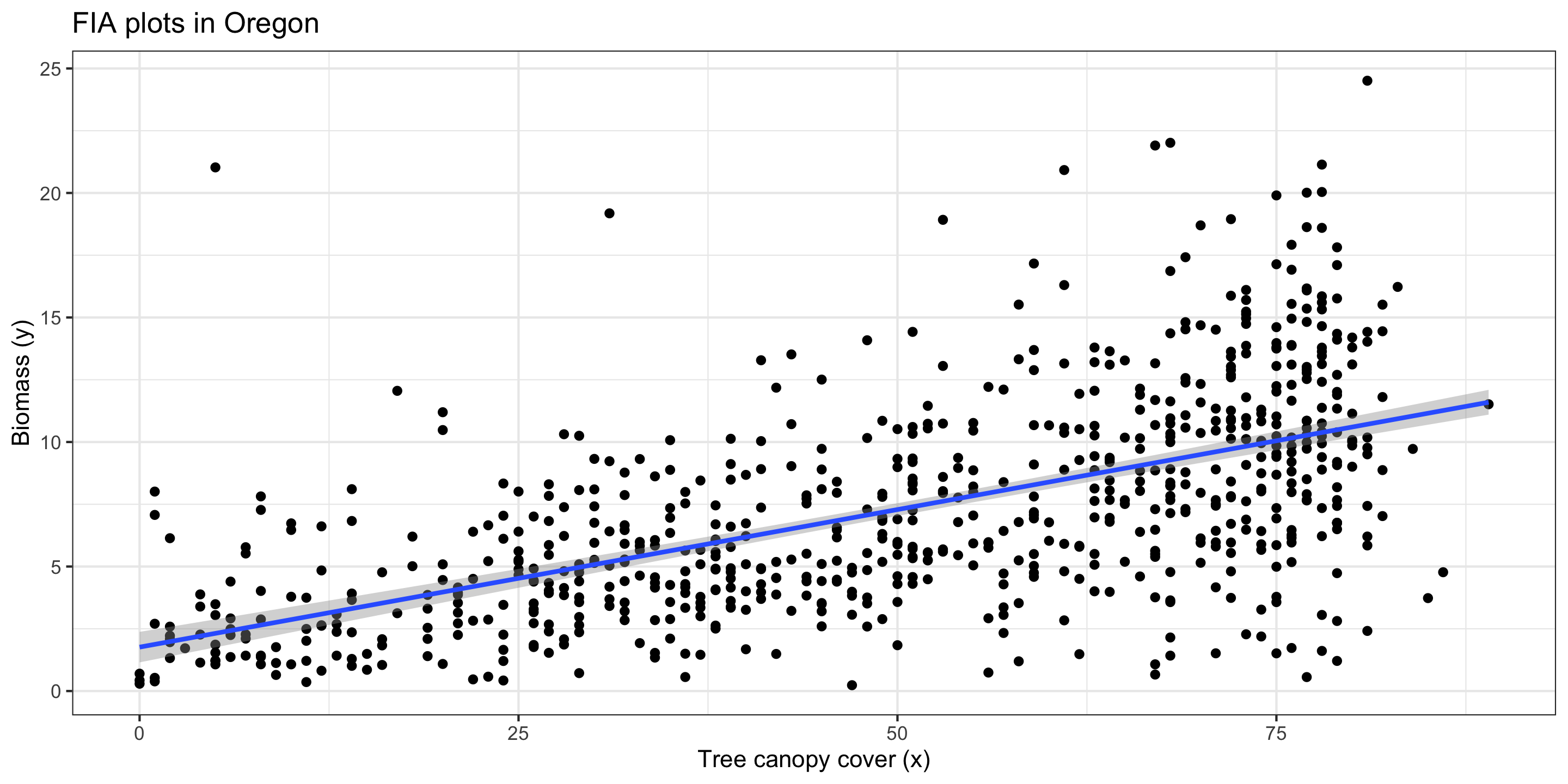
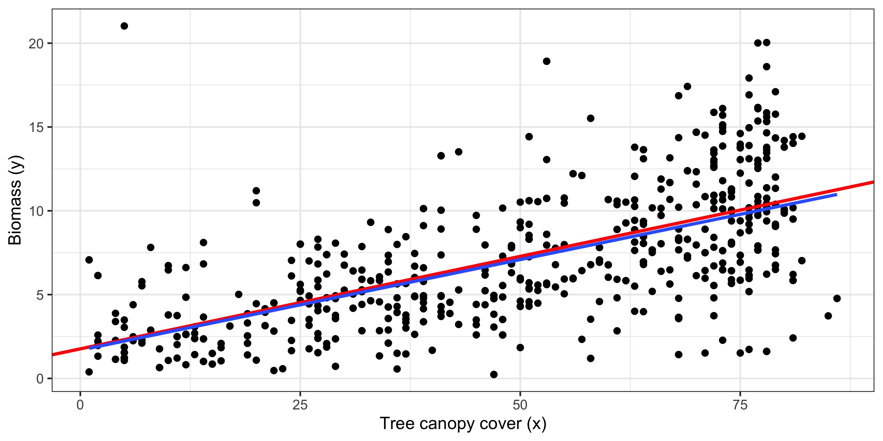
Plotting a Regression Line
Let’s add the regression line to our plot from before:
1) Linearity
Linearity: The relationship between explanatory and response variables must be approximately linear.

I think this assumption has been met.
3) Normality (of Residuals)
Normality of Residuals: The residuals should follow a normal distribution.
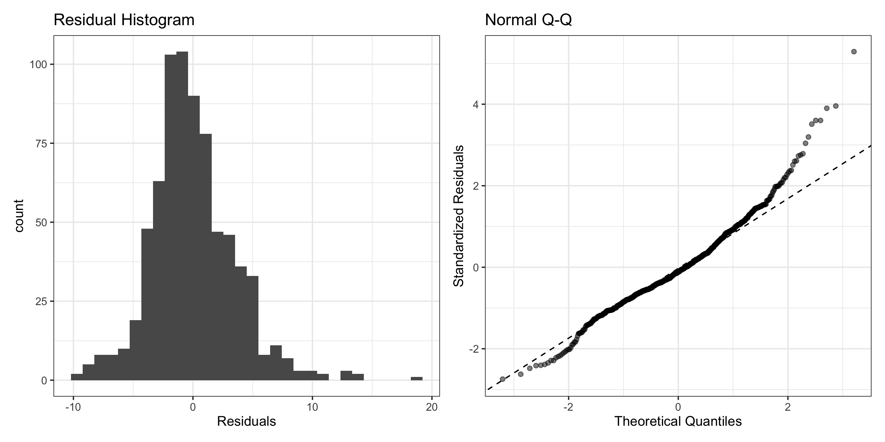
- Residuals aren’t quite Normal (right-skew, high outliers)
- Don’t discard all conclusions, but be skeptical in them.
I don’t think this assumption has been met.
4) Equal Variability (of Residuals)
Equal Variability: Variance of residuals should be roughly constant across data set.
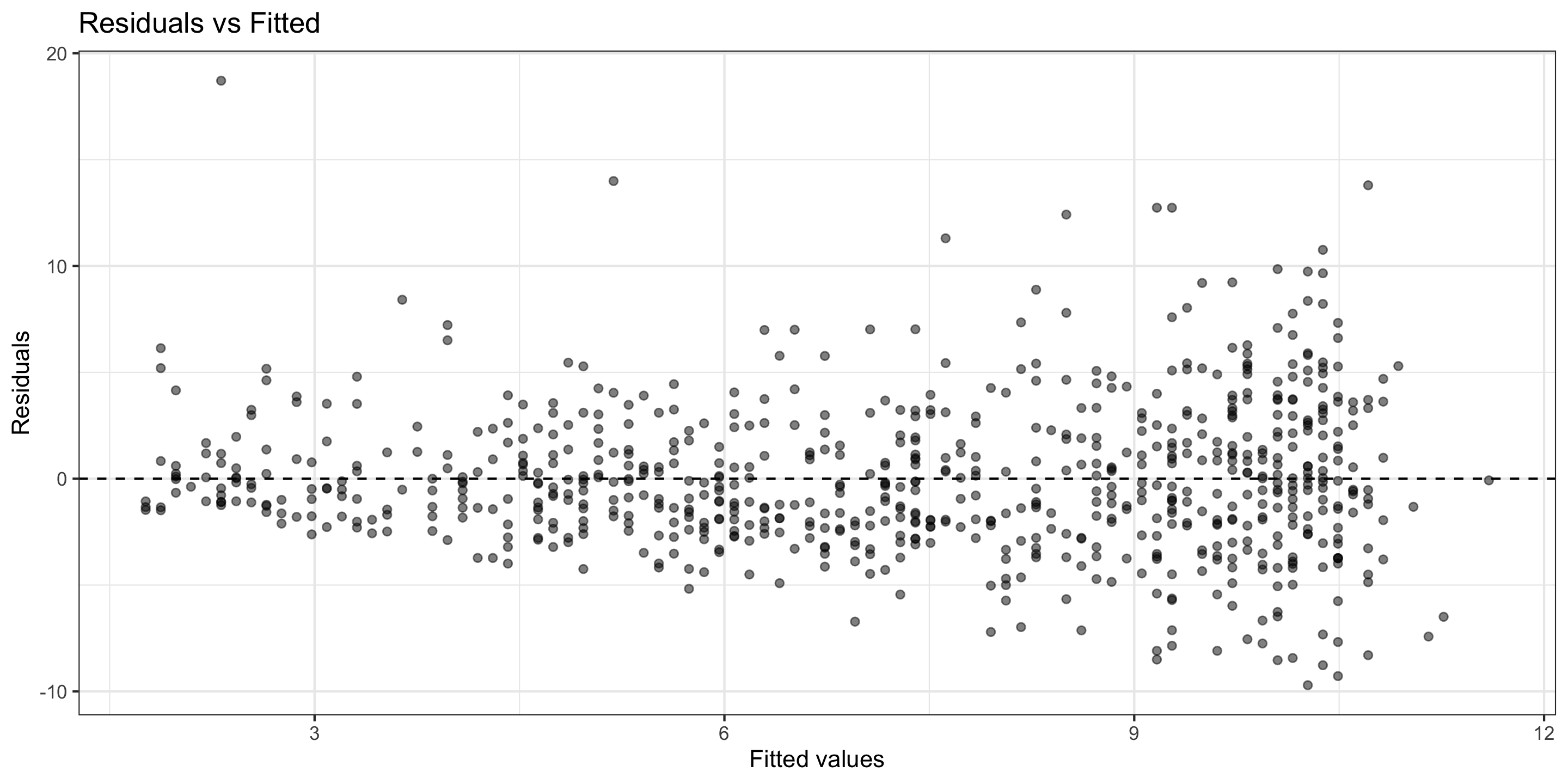
- There seems to be non-constant variability
- As canopy cover increases, the variance of the residuals increases.
I think this assumption is not met.
Bootstrapping in Regression
To approximate variability in our regression coefficients, \(\hat\beta_0\) and \(\hat\beta_1\) for this simple linear regression example, we bootstrap our sample!
- i.e., we sample, with replacement, rows from our original data.
- For each bootstrap sample, we calculate a new linear model
oregon %>%
  specify(biomass ~ canopy_cover) %>%
  generate(
    reps = 1,
    type = "bootstrap"
) 
Red line: Original regression line
Blue line: Bootstrap regression line
Bootstrapping in Regression
To approximate variability in our regression coefficients, \(\hat\beta_0\) and \(\hat\beta_1\) for this simple linear regression example, we bootstrap our sample!
- i.e., we sample, with replacement, rows from our original data.
- For each bootstrap sample, we calculate a new linear model
oregon %>%
  specify(biomass ~ canopy_cover) %>%
  generate(
    reps = 2,
    type = "bootstrap"
) 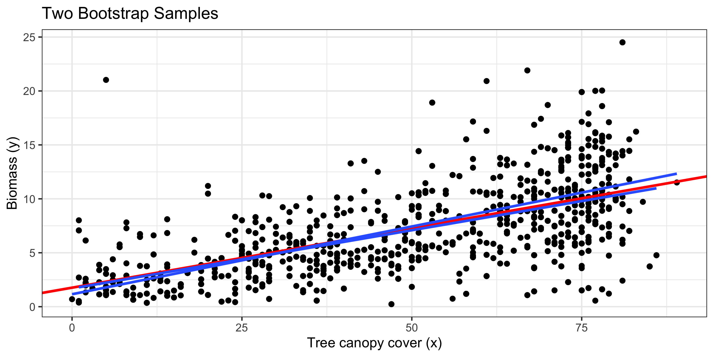
Red line: Original regression line
Blue line: Bootstrap regression line
Bootstrapping in Regression
To approximate variability in our regression coefficients, \(\hat\beta_0\) and \(\hat\beta_1\) for this simple linear regression example, we bootstrap our sample!
- i.e., we sample, with replacement, rows from our original data.
- For each bootstrap sample, we calculate a new linear model
oregon %>%
  specify(biomass ~ canopy_cover) %>%
  generate(
    reps = 1000,
    type = "bootstrap"
) 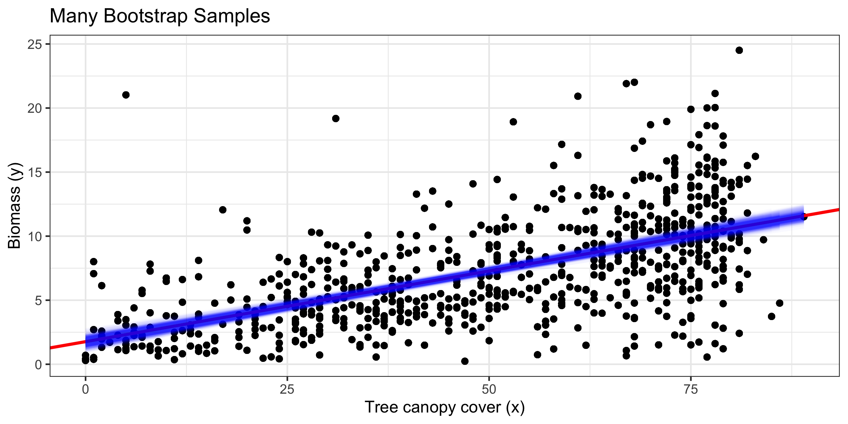
Red line: Original regression line
Blue line: Bootstrap regression line
Confidence intervals
We use the bootstrap distributions to produce confidence intervals.
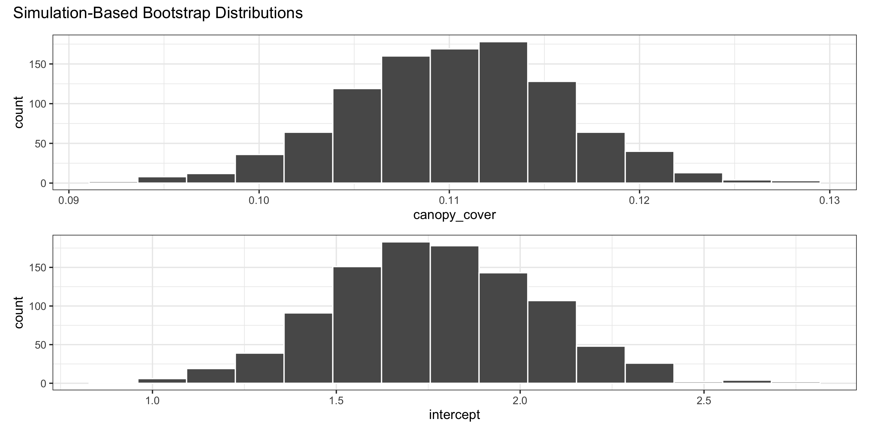
Confidence intervals
For the intercept:

Confidence intervals
For slopes:

Hypothesis Tests
Visualizing the null distribution and observed statistics
What’s wrong here?
Hypothesis Tests
Visualizing the null distribution and observed statistics
What’s wrong here?
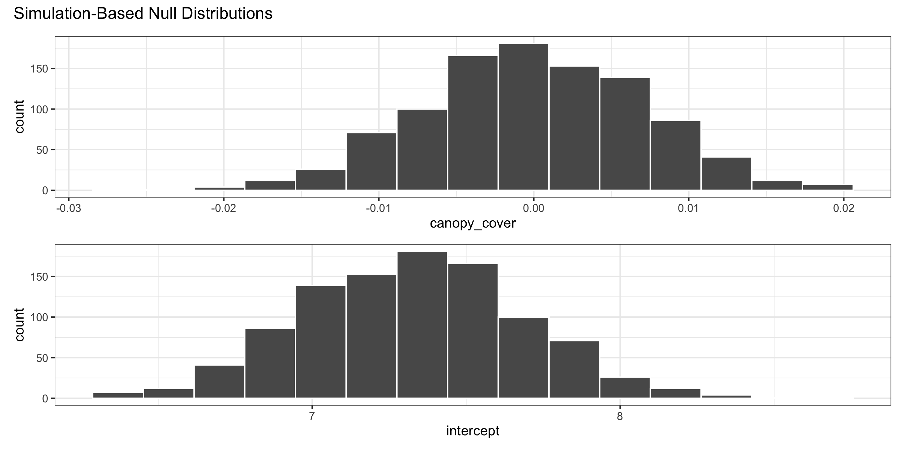
Hypothesis Tests for the intercept
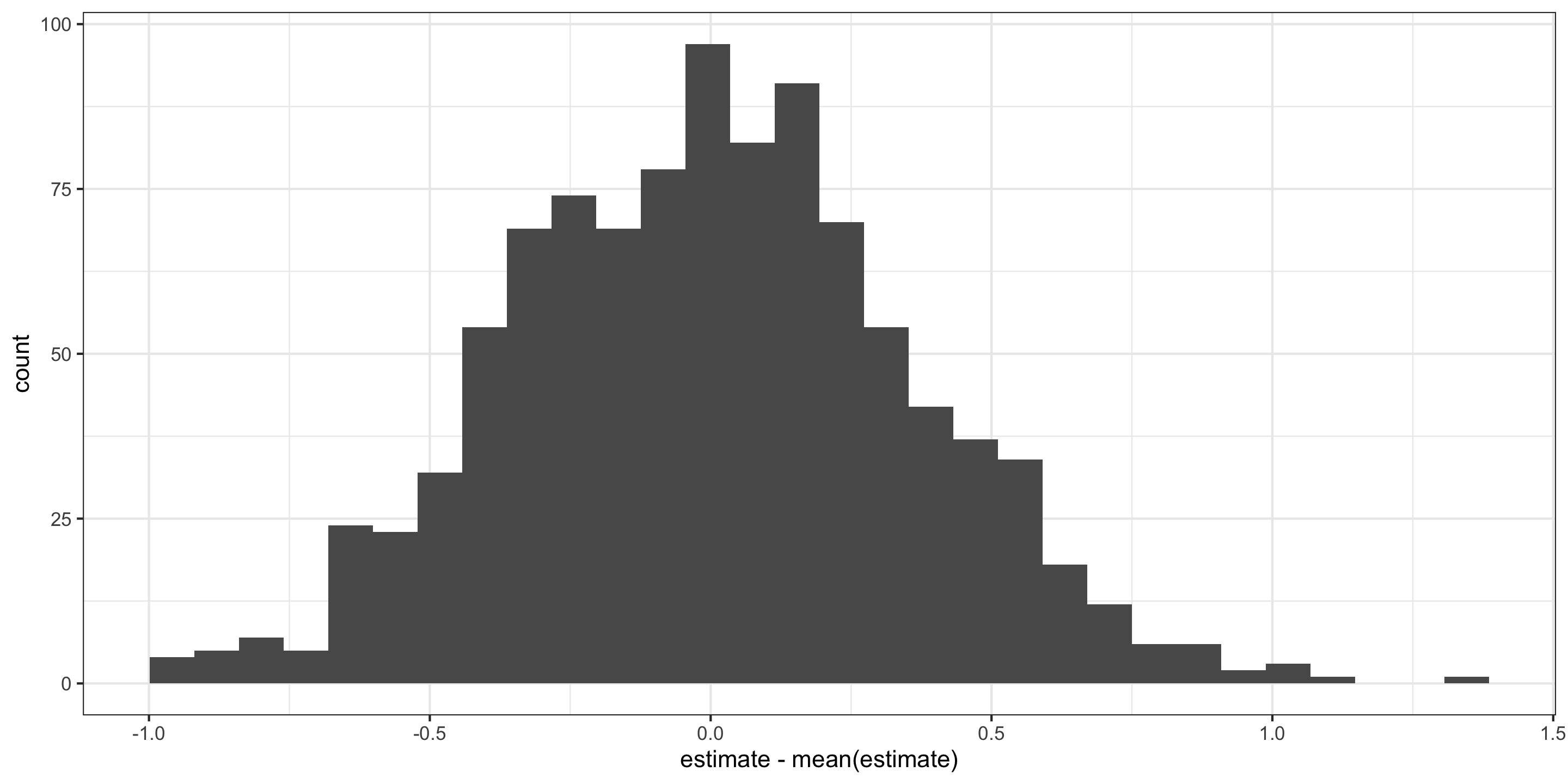
Visualizing the null distribution for the intercept “by hand”:
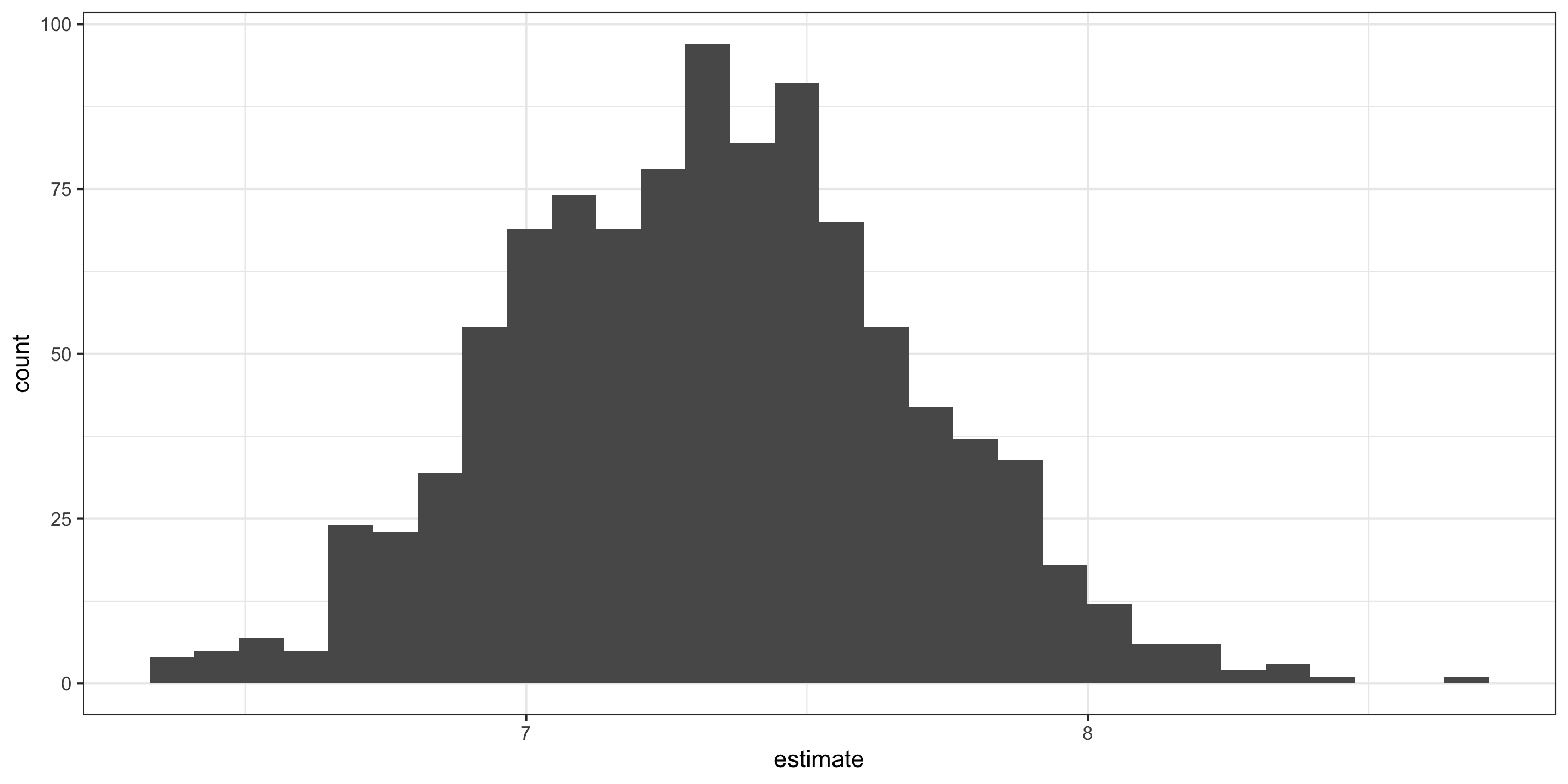
Hypothesis Tests for the intercept
Visualizing the null distribution for the intercept “by hand”:
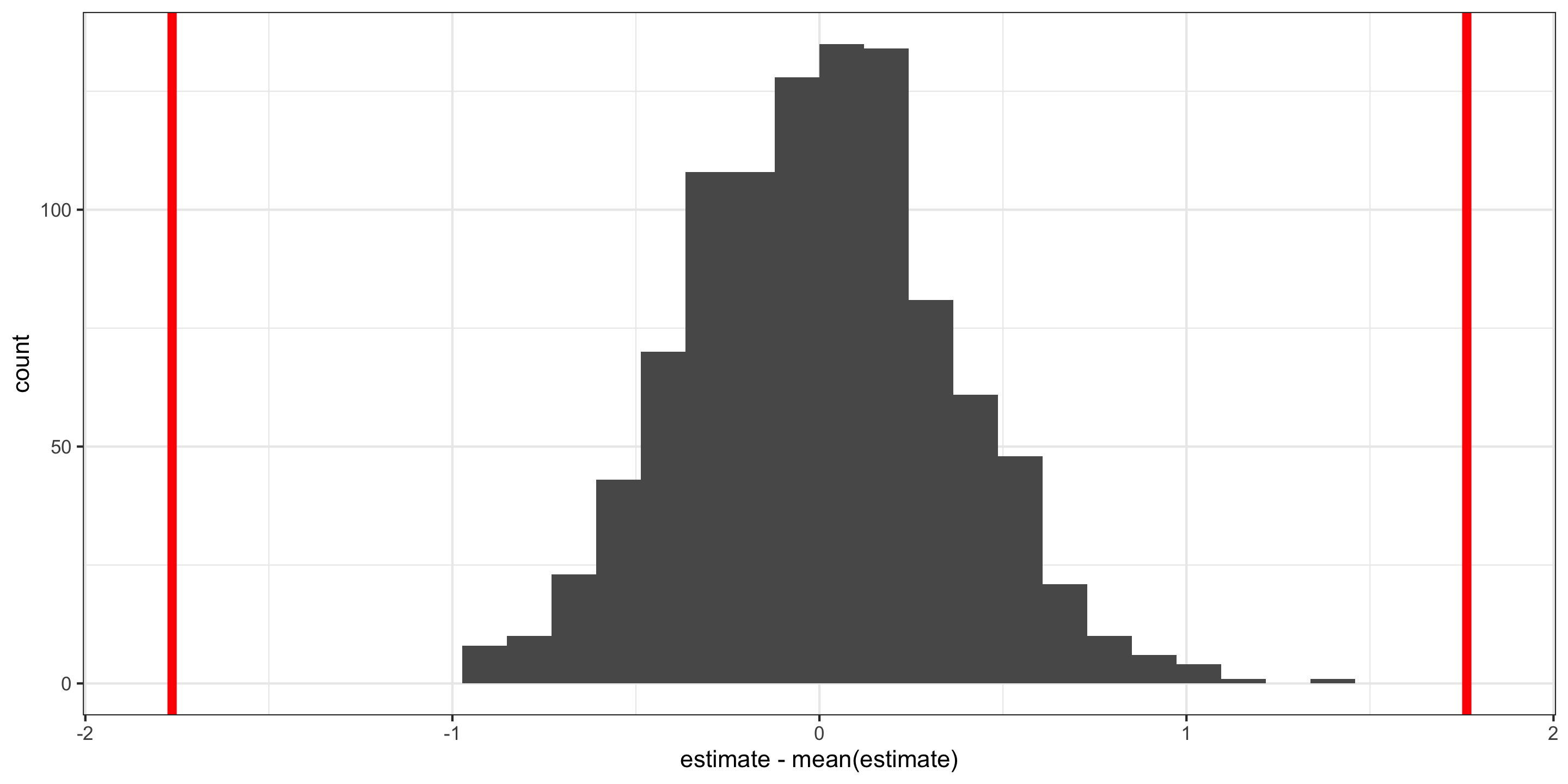
Hypothesis Tests for the intercept
Visualizing the null distribution and observed statistics, for the intercept, “by hand”:
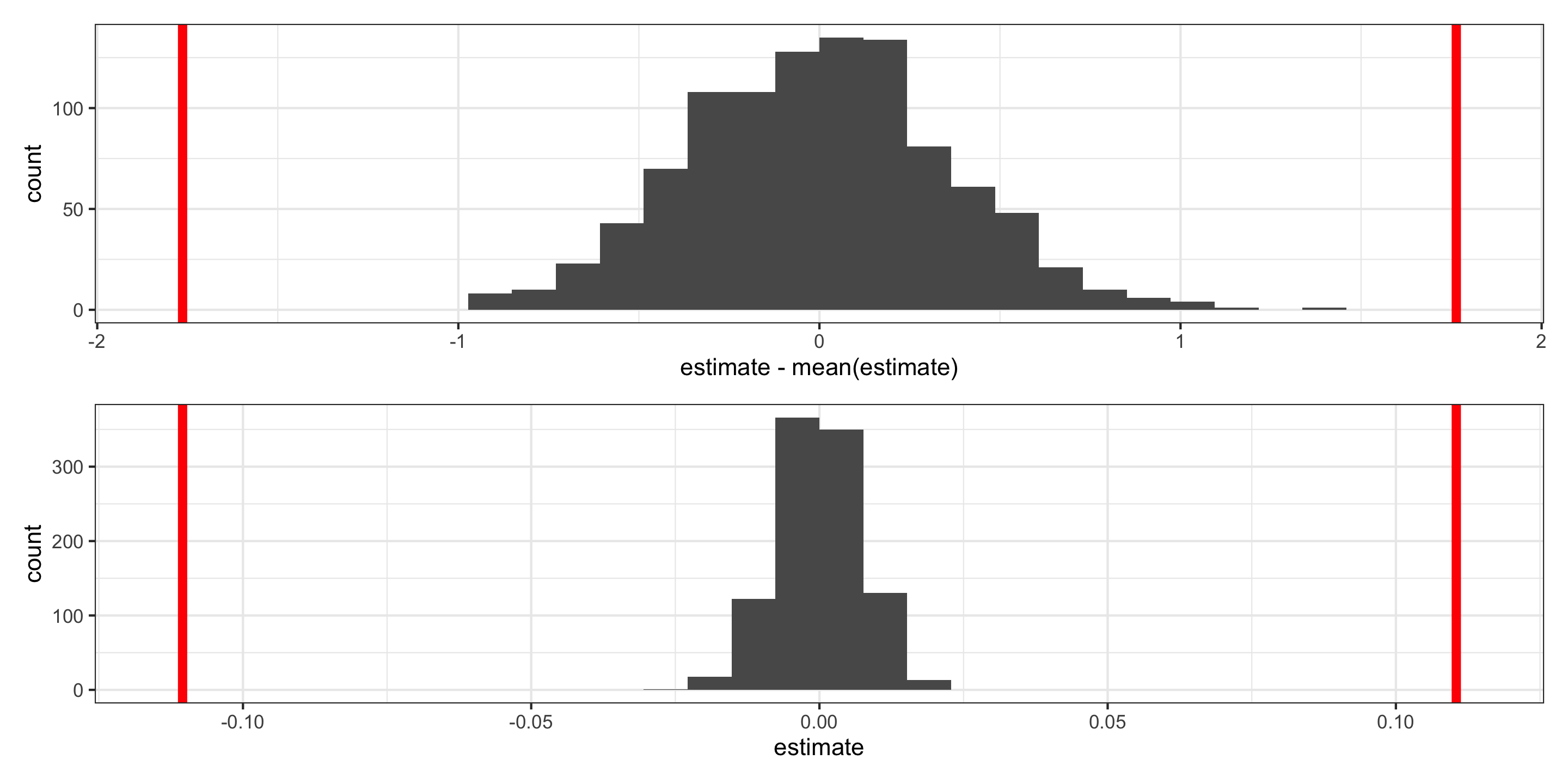
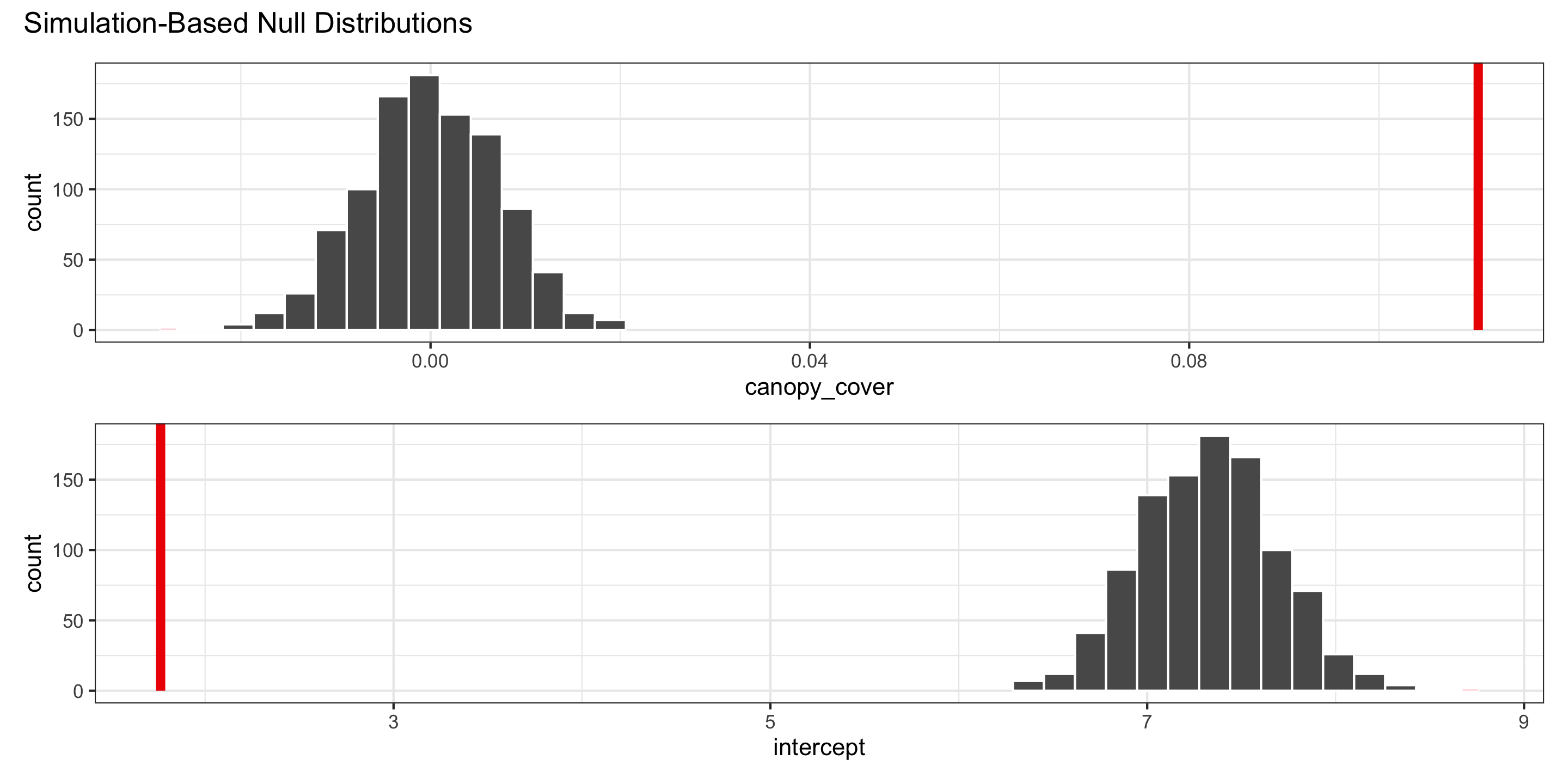
Hypothesis Tests
Visualizing the null distribution and observed statistics, for the intercept:
p1 <- null %>%
  filter(term == "intercept") %>%
  ggplot(aes(x = estimate - mean(estimate))) +
  geom_histogram() +
  geom_vline(xintercept = obs_stats$estimate[1], color = "red", size = 2) +
  geom_vline(xintercept = -obs_stats$estimate[1], color = "red", size = 2)

p2 <- null %>%
  filter(term == "canopy_cover") %>%
  ggplot(aes(x = estimate)) +
  geom_histogram() +
  geom_vline(xintercept = obs_stats$estimate[2], color = "red", size = 2) +
  geom_vline(xintercept = -obs_stats$estimate[2], color = "red", size = 2)

p1 / p2