Regression Inference III and ANOVA


Grayson White

Math 141
Week 13 | Fall 2025

Announcements

  • Don’t forget to sign up for an oral exam slot!

Goals for Today

  • Discuss inference for regression with categorical variables.
  • Introduce the ANOVA test.
  • Learn about the F distribution.

Example

Do Audience Ratings vary by movie genre?

library(tidyverse)
# Load data
library(Lock5Data)
movies <- HollywoodMovies2011 %>%
  filter(!(Genre %in% c("Fantasy", "Adventure"))) %>%
  drop_na(Genre, AudienceScore)
  • Cases:

  • Variables of interest (including type):

  • Hypotheses:

Example

Does there appear to be a relationship?

ggplot(data = movies, 
       mapping = aes(x = Genre,
                     y = AudienceScore)) + 
  geom_boxplot() +     
  stat_summary(fun = mean, geom = "point", 
               color = "purple",
               shape = 8, size = 3)

  • What movie did the audience hate so much??

Example

Does there appear to be a relationship?

bad <- filter(movies, 
        AudienceScore == min(AudienceScore))
ggplot(data = movies, 
       mapping = aes(x = Genre,
                     y = AudienceScore)) + 
  geom_boxplot() +     
  stat_summary(fun = mean, geom = "point", 
               color = "purple",
               shape = 8, size = 3) +
  geom_label(data = bad, 
             mapping = aes(label = Movie))

What movie did the audience hate so much??

Trespass

Okay, how could we answer our original question?

Do Audience Ratings vary by movie genre?

Let’s do inference for regression to find out!

# fit the model
mod <- lm(AudienceScore ~ Genre, movies)
get_regression_table(mod)
# A tibble: 7 × 7
  term             estimate std_error statistic p_value lower_ci upper_ci
  <chr>               <dbl>     <dbl>     <dbl>   <dbl>    <dbl>    <dbl>
1 intercept          58.6        2.80    20.9     0        53.1    64.2  
2 Genre: Animation    5.46       5.37     1.02    0.311    -5.16   16.1  
3 Genre: Comedy       0.486      4.14     0.117   0.907    -7.71    8.68 
4 Genre: Drama       13.5        4.45     3.03    0.003     4.66   22.3  
5 Genre: Horror      -9.98       4.76    -2.10    0.038   -19.4    -0.562
6 Genre: Romance      6.18       5.74     1.08    0.284    -5.19   17.5  
7 Genre: Thriller     5.68       5.21     1.09    0.278    -4.64   16.0  

What tests are occurring here?

\(H_o: \beta_j = 0\), \(H_A: \beta_j \neq 0\). For \(j > 0\), we are testing if there is a difference from the baseline group. For \(j = 0\) we are testing if the baseline group is different than 0.

What sort of test might we want to carry out more often?

Inference for Many Means

Inference for Many Means

Consider the situation where:

  • Response variable: quantitative

  • Explanatory variable: categorical

  • Parameter of interest: \(\mu_1 - \mu_2\)

  • This parameter of interest only makes sense if the explanatory variable is restricted to two categories.

  • Can use linear regression but in the special case of categorical explanatory variables, we have another option.

    • It is time to learn how to conduct inference for more than two means.

Hypotheses

Consider the situation where:

  • Response variable: quantitative

  • Explanatory variable: categorical

\(H_o\): \(\mu_1 = \mu_2 = \cdots = \mu_K\) (Variables are independent/not related.)

\(H_a\): At least one mean is not equal to the rest. (Variables are dependent/related)

Example

Do Audience Ratings vary by movie genre?

library(tidyverse)
# Load data
library(Lock5Data)
movies <- HollywoodMovies2011 %>%
  filter(!(Genre %in% c("Fantasy", "Adventure"))) %>%
  drop_na(Genre, AudienceScore)
  • Cases:

  • Variables of interest (including type):

  • Hypotheses:

Test Statistic

Need a test statistic!

  • Won’t be a sample statistic.

\[ \bar{x}_1 - \bar{x}_2 - \cdots - \bar{x}_K \mbox{ won't work!} \]

  • Needs to measure the discrepancy between the observed sample and the sample we’d expect to see if \(H_o\) were true.

  • Would be nice if its null distribution could be approximated by a known probability model.

We’ll consider a test called “ANOVA”

  • Called “Analysis of VARIANCE” test.

  • Not called “Analysis of MEANS” test.

  • Question: Why analyze variability to test differences in means?

Why analyze variability to test differences in means?

Let’s look at some simulated data for a moment.

Question: For which scenario are you most convinced that the means are different?

Key Idea: Partitioning the Variability

\[\begin{align*} & \mbox{Total Variability} = \\ & \mbox{Variability Between Groups} + \\ & \mbox{Variability Within Groups} \end{align*}\]

  • Variability Between Groups: How much the group means vary
    • Compare the red dots.
  • Variability Within Groups: How much natural group variability there is
    • Within groups, compare the black dots to the red dot.

Key Idea: Partitioning the Variability

  • Total Variability: How much points vary from the overall mean

\[\begin{align*} \mbox{Total Variability} &= \sum_{i=1}^n (x_i - \bar{x})^2 \\ & = \mbox{Sum of Squares Total} \\ & = \mbox{SSTotal} \end{align*}\]

Key Idea: Partitioning the Variability

  • Variability Between Groups: How much the group means vary
    • Compare the red dots.

\[\begin{align*} \mbox{Variability Between Groups} &= \sum_{k = 1}^K n_k (\bar{x}_k - \bar{x})^2 \\ & = \mbox{Sum of Squares Group} \\ & = \mbox{SSG} \end{align*}\]

Key Idea: Partitioning the Variability

  • Variability Within Groups: How much natural group variability there is
    • Within groups, compare the black dots to the red dot.

\[\begin{align*} \mbox{Variability Within Groups} &= \sum_{k = 1}^{K} \sum_{i = 1}^{n_k} (x_{ik} - \bar{x}_k)^2 \\ & = \mbox{Sum of Squares Error} \\ & = \mbox{SSE} \end{align*}\]

\[\begin{align*} \mbox{Total Variability} & = \mbox{Variability Between Groups} + \mbox{Variability Within Groups} \end{align*}\]

Mean Squares

Need to standardize the Sums of Squares to compare SSG to SSE.

\[\begin{align*} \mbox{Mean Variability Between Groups} & = \frac{\mbox{SSG}}{K - 1} = MSG \end{align*}\]

\[\begin{align*} \mbox{Mean Variability Within Groups} & = \frac{\mbox{SSE}}{n - K} = MSE \end{align*}\]

  • Now on a comparable scale!

  • Now we can create a test statistic that compares these two measures of variability.

Test Statistic

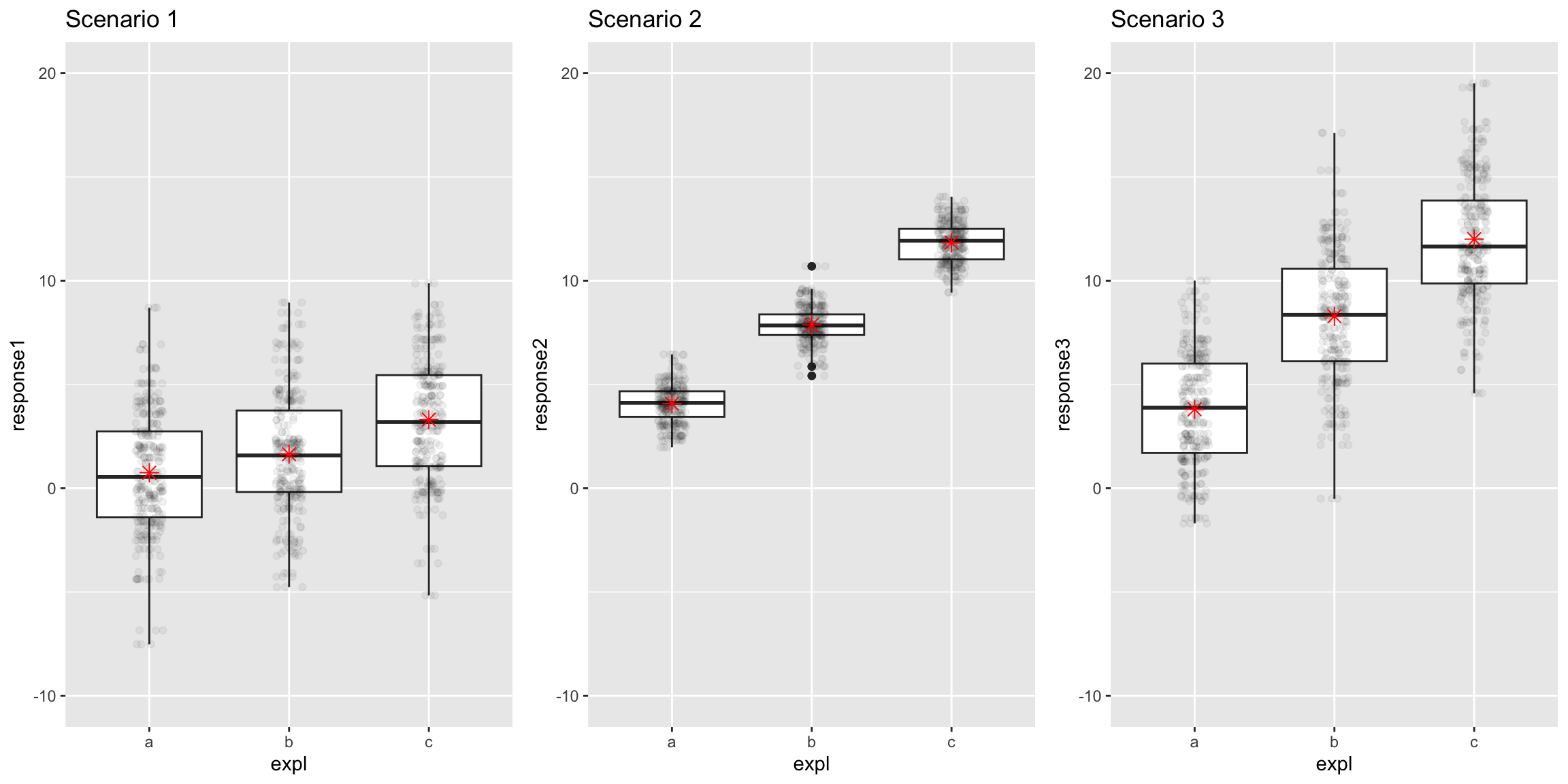
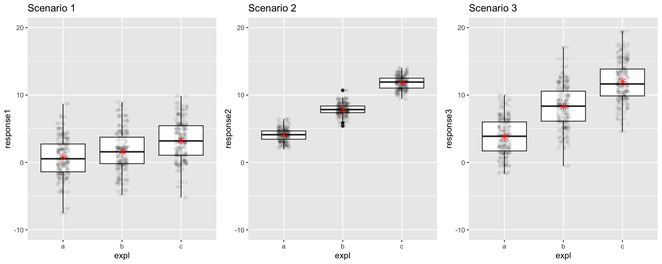
In some ways, MSG is the natural test statistic but as we saw for this example, MSG alone isn’t enough.

  • Scenarios 2 and 3 have roughly the same MSG but we are much more convinced that the means are different for 2 than 3.

  • That is where MSE comes in!
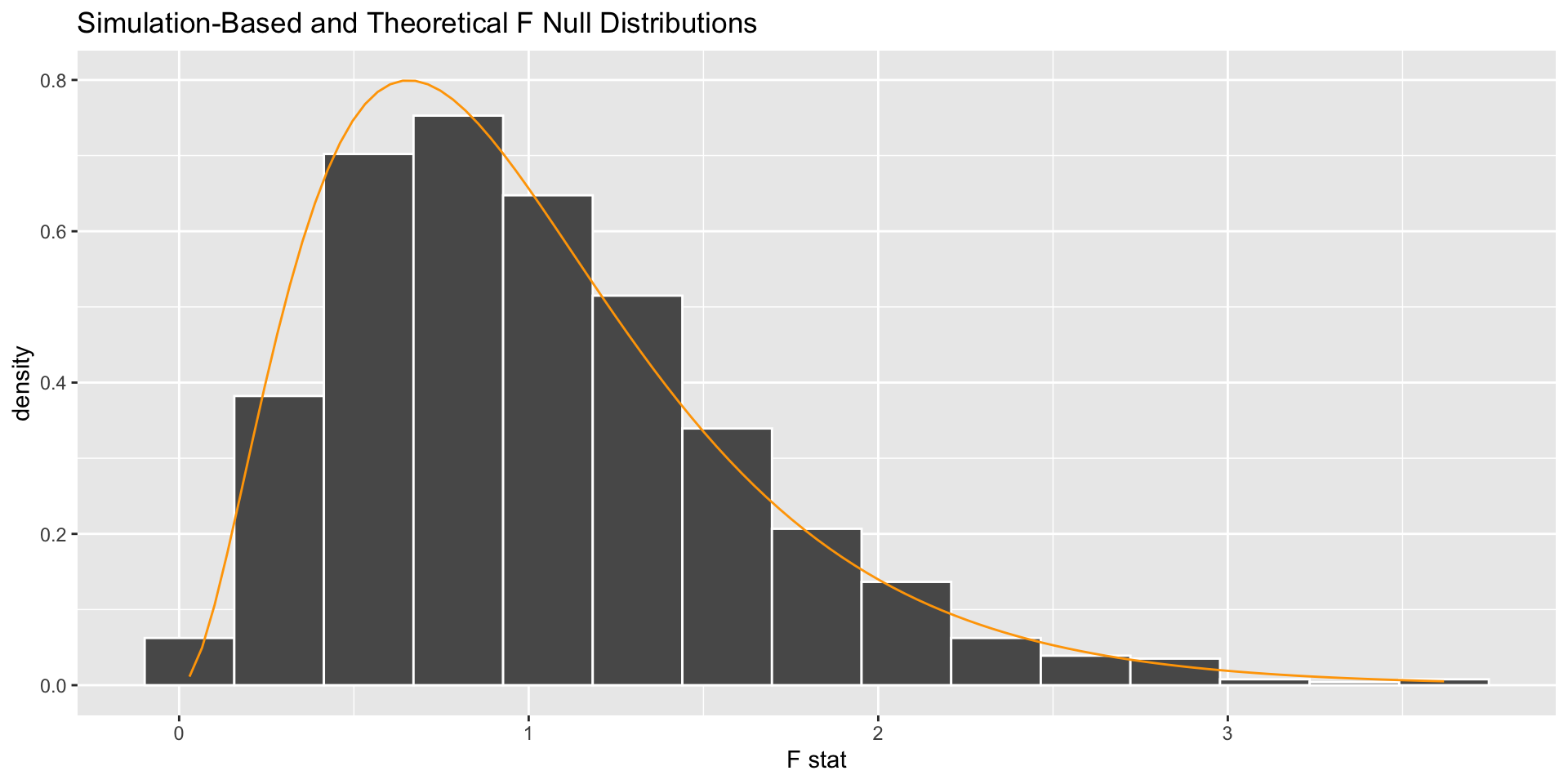
Test Statistic

\[ F = \frac{\mbox{MSG}}{\mbox{MSE}} = \frac{\mbox{variance between groups}}{\mbox{variance within groups}} \]

  • If \(H_o\) is true, then \(F\) should be roughly equal to what?

  • If \(H_a\) is true, then \(F\) should be greater than 1 because there is more variation in the group means than we’d expect if the population means are all equal.

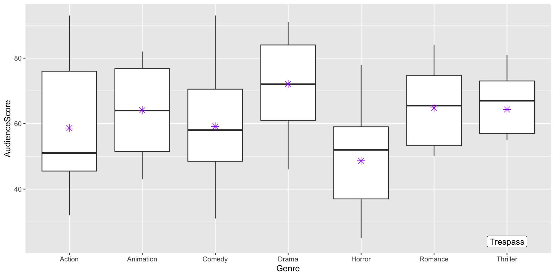
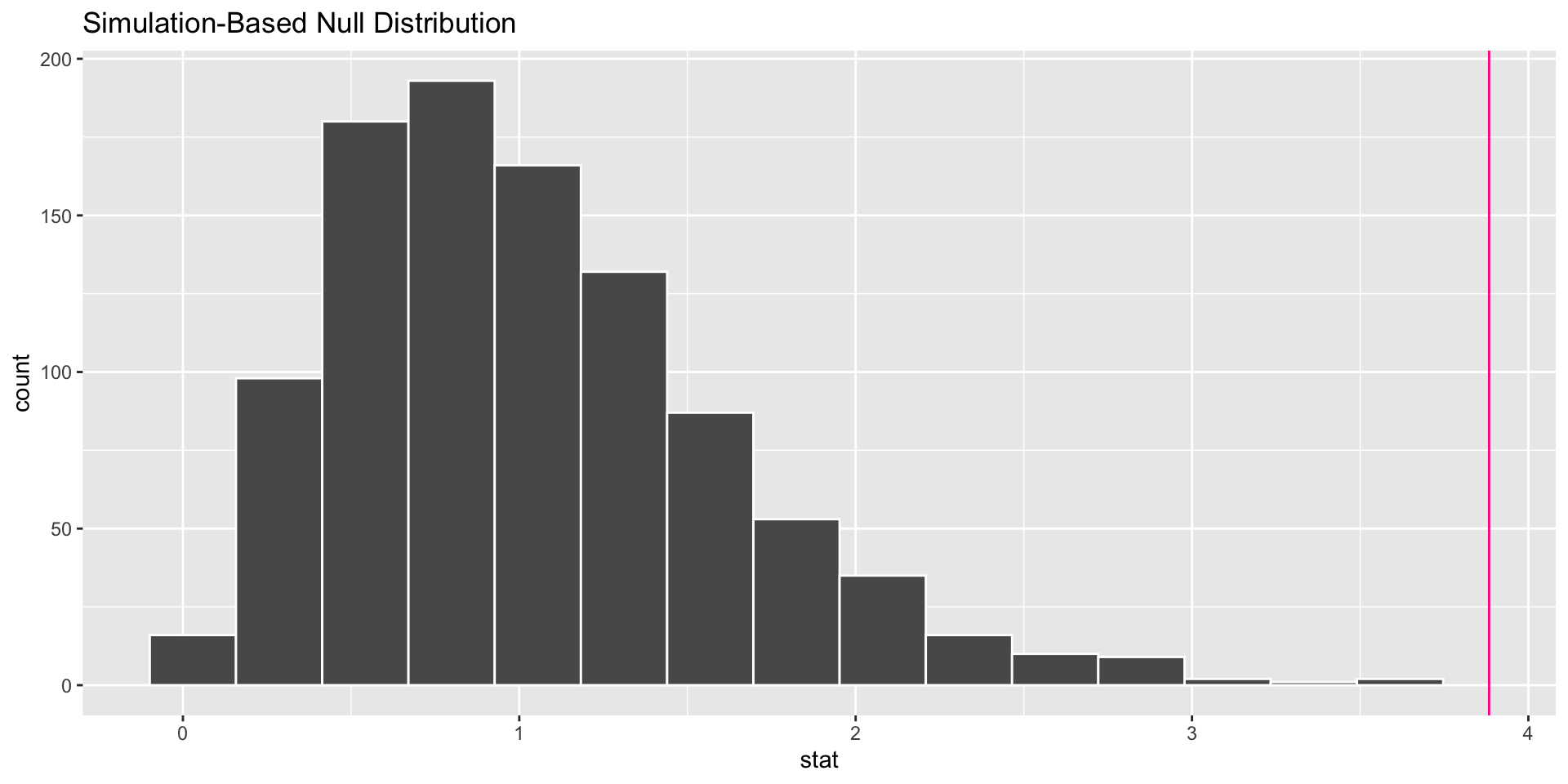
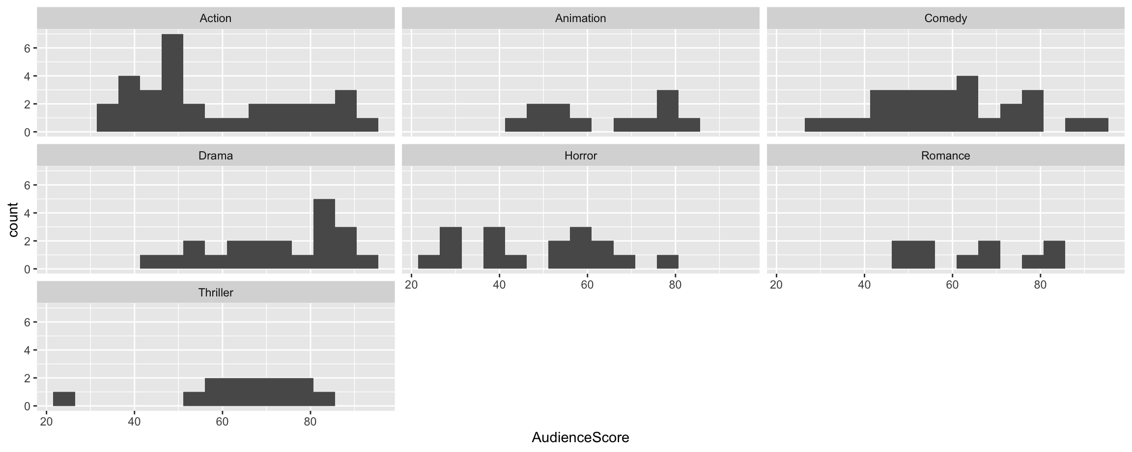
Returning to the Movies Example

library(infer)
#Compute F test stat
test_stat <- movies %>%
  specify(AudienceScore ~ Genre) %>%
  calculate(stat = "F") 
test_stat
Response: AudienceScore (numeric)
Explanatory: Genre (factor)
# A tibble: 1 × 1
   stat
  <dbl>
1  3.88
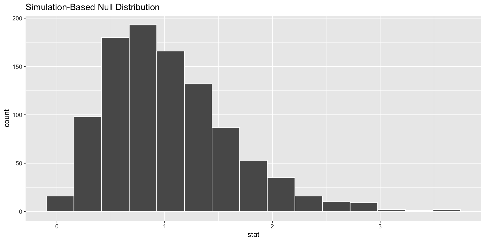
  • Is 3.88 a large test statistic? Is a test statistic of 3.88 unusual under \(H_o\)?

Generating the Null Distribution

   AudienceScore     Genre
1             63  Thriller
2             34    Action
3             39    Action
4             49    Comedy
5             38    Horror
6             68     Drama
7             55    Action
8             31    Comedy
9             91     Drama
10            70  Thriller
11            63   Romance
12            53     Drama
13            73 Animation
14            42    Comedy
15            76 Animation
16            63    Comedy
17            54    Comedy
18            55    Comedy
19            59 Animation
20            77    Comedy

Steps:

  1. Shuffle Genre.
  2. Compute the \(MSE\) and \(MSG\).
  3. Compute the test statistic.
  4. Repeat 1 - 3 many times.

Generating the Null Distribution

# Construct null distribution
null_dist <- movies %>%
  specify(AudienceScore ~ Genre) %>%
  hypothesize(null = "independence") %>%
  generate(reps = 1000, type = "permute") %>%
  calculate(stat = "F") 
visualize(null_dist)

The Null Distribution

Key Observations:

  • Smallest possible value?


  • Shape?

The Null Distribution

Key Observations:

  • Is our observed test statistic unusual?

The P-value

# Compute p-value
null_dist %>%
  get_pvalue(obs_stat = test_stat, direction = "greater")
# A tibble: 1 × 1
  p_value
    <dbl>
1       0

Approximating the Null Distribution

If

  • There are at least 30 observations in each group or the response variable is normal
  • The variability is similar for all groups

then

\[ \mbox{test statistic} \sim F(df1 = K - 1, df2 = n - K) \]

The ANOVA Test

Check assumptions!

movies %>%
  group_by(Genre) %>%
  summarize(n(), sd(AudienceScore))
# A tibble: 7 × 3
  Genre     `n()` `sd(AudienceScore)`
  <fct>     <int>               <dbl>
1 Action       32                18.4
2 Animation    12                13.9
3 Comedy       27                15.7
4 Drama        21                14.5
5 Horror       17                15.9
6 Romance      10                12.9
7 Thriller     13                14.9

The ANOVA Test

Check assumptions!

ggplot(data = movies, mapping = aes(x = AudienceScore)) + 
  geom_histogram(bins = 15) + 
  facet_wrap(~Genre)

The ANOVA Test

mod_anova <- aov(AudienceScore ~ Genre, data = movies)
summary(mod_anova)
             Df Sum Sq Mean Sq F value Pr(>F)   
Genre         6   5855     976    3.88 0.0014 **
Residuals   125  31413     251                  
---
Signif. codes:  0 '***' 0.001 '**' 0.01 '*' 0.05 '.' 0.1 ' ' 1

Many ANOVA Tests Out There!

  • We learned the One-Way ANOVA test.

  • Two-Way: Have two categorical, explanatory variables.

  • Repeated Measures ANOVA: Have multiple observations on each case.

    • All the tests we have focused on assumed independent observations.
  • ANOVA Tests for Regression: Allow comparisons of various subsets of a multiple linear regression model.

Next time: more categorical variable inference