Chi-squared test of independence

Grayson White

Math 141
Week 13 | Fall 2025

Goals for Today

Chi-squared tests

Chi-squared distribution

Continuing our Discussion of Moving Beyond BINARY Categorical Variables

Inference for Categorical Variables

Consider the situation where:

Response variable: categorical
Explanatory variable: categorical
Parameter of interest: \(p_1 - p_2\)
- This parameter of interest only makes sense if both variables only have two categories.

It is time to learn how to study the relationship between two categorical variables when at least one has more than two categories.

Hypotheses

\(H_o\): The two variables are independent.

\(H_a\): The two variables are dependent.

Example

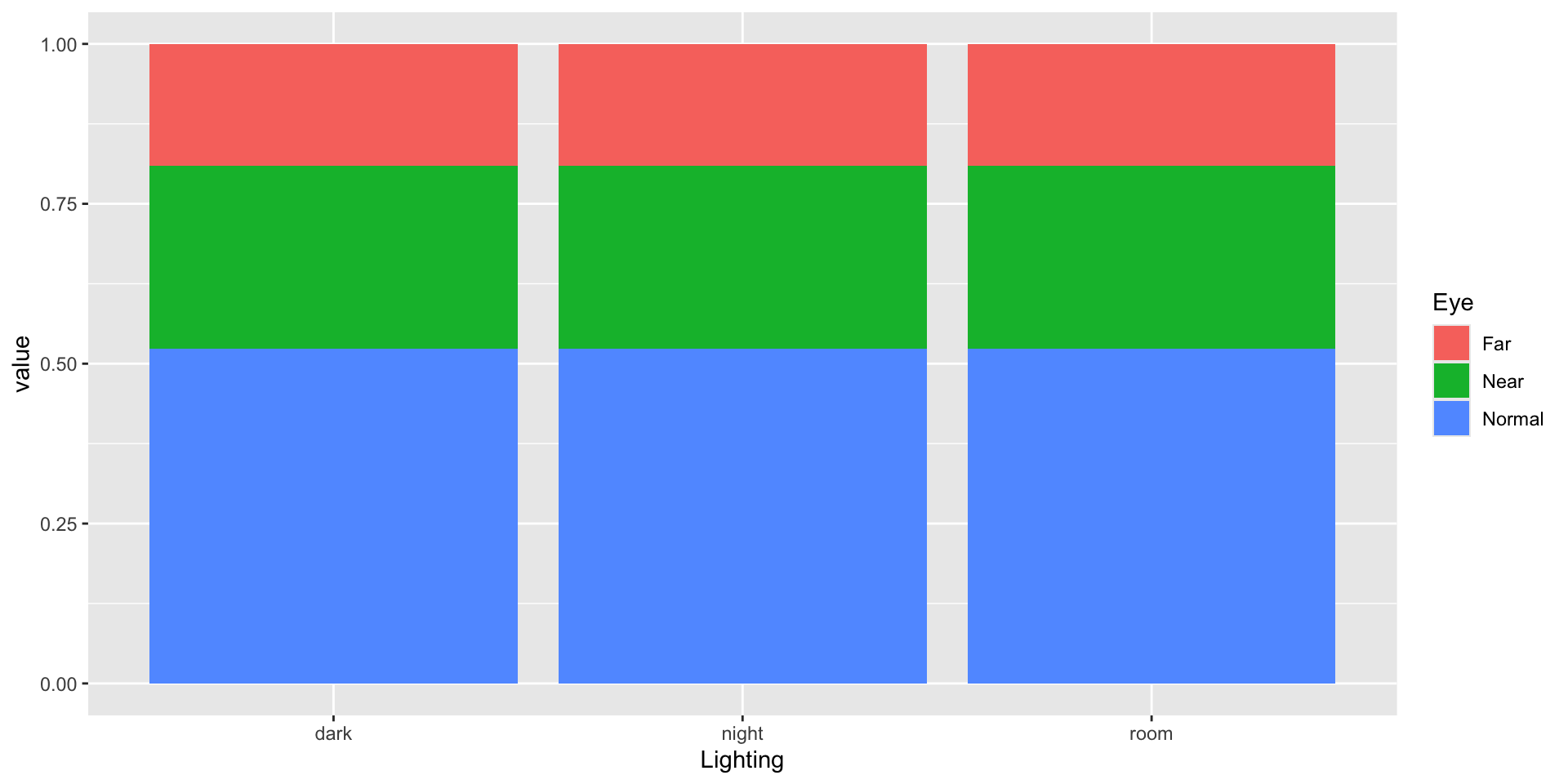
Near-sightedness typically develops during the childhood years. Quinn, Shin, Maguire, and Stone (1999) explored whether there is a relationship between the type of light children were exposed to and their eye health based on questionnaires filled out by the children’s parents at a university pediatric ophthalmology clinic.

library(tidyverse)
library(infer)

# Import data
eye_data <- read_csv("data/eye_lighting.csv")

# Contingency table
eye_data %>%
  count(Lighting, Eye)

# A tibble: 9 × 3
  Lighting Eye        n
  <chr>    <chr>  <int>
1 dark     Far       40
2 dark     Near      18
3 dark     Normal   114
4 night    Far       39
5 night    Near      78
6 night    Normal   115
7 room     Far       12
8 room     Near      41
9 room     Normal    22

Eyesight Example

Does there appear to be a relationship/dependence?

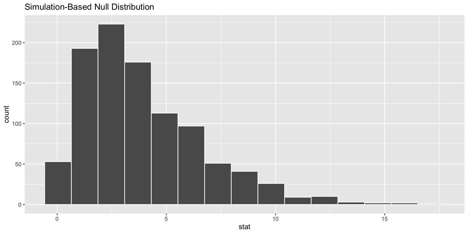
ggplot(data = eye_data, 
       mapping = aes(x = Lighting,
                     fill = Eye)) + 
  geom_bar(position = "fill")

Test Statistic

Need a test statistic!

Won’t be a single sample statistic.
Needs to measure the discrepancy between the observed sample and the sample we’d expect to see if \(H_o\) (no relationship) were true.
Would be nice if its null distribution could be approximated by a known probability model.

Sample Result Tables

Observed Sample Table

table(eye_data$Eye, eye_data$Lighting) %>%
  addmargins() %>%
  kable(format = "html")

	dark	night	room	Sum
Far	40	39	12	91
Near	18	78	41	137
Normal	114	115	22	251
Sum	172	232	75	479

Expected Sample Table

Question: If \(H_o\) were correct, is this the table that we’d expect to see?

	dark	night	room	Sum
Far	53	53	53	159
Near	53	53	53	159
Normal	53	53	53	159
Sum	159	159	159	477

Sample Result Tables

Observed Sample Table

table(eye_data$Eye, eye_data$Lighting) %>%
  addmargins() %>%
  kable(format = "html")

	dark	night	room	Sum
Far	40	39	12	91
Near	18	78	41	137
Normal	114	115	22	251
Sum	172	232	75	479

Expected Sample Table

Question: If \(H_o\) were correct, what table would we expect to see?

Want a \(H_o\) table that respects the overall eye condition proportions:

\[\hat{p}_{far} = 91/479\]

\[\hat{p}_{nor} = 251/479\]

\[\hat{p}_{nea} = 137/479\]

Sample Result Tables

Observed Sample Table

table(eye_data$Eye, eye_data$Lighting) %>%
  addmargins() %>%
  kable(format = "html")

	dark	night	room	Sum
Far	40	39	12	91
Near	18	78	41	137
Normal	114	115	22	251
Sum	172	232	75	479

Expected Sample Table

Question: If \(H_o\) were correct, what table would we expect to see?

	dark	night	room	Sum
Far	(91/479)172	(91/479)232	(91/479)75	91
Near	(137/479)172	(137/479)232	(137/479)75	137
Normal	(251/479)172	(251/479)232	(251/479)75	251
Sum	172	232	75	479

Still have the same totals but distributed the values differently within the table

Sample Result Tables

Observed Sample Table

table(eye_data$Eye, eye_data$Lighting) %>%
  addmargins() %>%
  kable(format = "html")

	dark	night	room	Sum
Far	40	39	12	91
Near	18	78	41	137
Normal	114	115	22	251
Sum	172	232	75	479

Expected Sample Table

Question: If \(H_o\) were correct, what table would we expect to see?

	dark	night	room	Sum
Far	33	44	14	91
Near	49	66	22	137
Normal	90	122	39	251
Sum	172	232	75	479

Expected Table

How does this table represent \(H_o\)?

	dark	night	room	Sum
Far	33	44	14	91
Near	49	66	21	137
Normal	90	122	39	251
Sum	172	232	75	479

Test Statistic

Want the test statistic to quantify the difference between the observed table and the expected table.

	dark	night	room	Sum
Far	40	39	12	91
Near	18	78	41	137
Normal	114	115	22	251
Sum	172	232	75	479

	dark	night	room	Sum
Far	32.68	44.08	14.25	91
Near	49.19	66.35	21.45	137
Normal	90.13	121.57	39.30	251
Sum	172.00	232.00	75.00	479

For each cell: Compute a Z-score!

\[\begin{align*} \mbox{Z-score} &= \frac{\mbox{stat - mean}}{\mbox{SE}} \\ & = \frac{\mbox{observed - expected}}{\sqrt{\mbox{expected}}} \end{align*}\]

Test Statistic

Want the test statistic to quantify the difference between the observed table and the expected table.

	dark	night	room
Far	1.3	-0.76	-0.6
Near	-4.5	1.43	4.2
Normal	2.5	-0.60	-2.8

Test Statistic

Test Statistic Formula:

\[\begin{align*} \chi^2 = \sum \left(\frac{\mbox{observed - expected}}{\sqrt{\mbox{expected}}} \right)^2 \end{align*}\]

library(infer)
#Compute Chi-square test stat
test_stat <- eye_data %>%
  specify(Eye ~ Lighting) %>%
  calculate(stat = "Chisq") 
test_stat

Response: Eye (factor)
Explanatory: Lighting (factor)
# A tibble: 1 × 1
   stat
  <dbl>
1  56.5

Questions:

Is a test statistic unusual if it is a large number or a small number?
Is 56.5 unusual under \(H_o\)?

Generating the Null Distribution

# Construct null distribution
null_dist <- eye_data %>%
  specify(Eye ~ Lighting) %>%
  hypothesize(null = "independence") %>%
  generate(reps = 1000, type = "permute") %>%
  calculate(stat = "Chisq")


visualize(null_dist)

The Null Distribution

Key Observations about the distribution:

Smallest possible value?

Shape?

Is our observed test statistic of 56.5 unusual?

The P-value

# Compute p-value
null_dist %>%
  get_pvalue(obs_stat = test_stat, direction = "greater")

# A tibble: 1 × 1
  p_value
    <dbl>
1       0

Approximating the Null Distribution

If there are at least 5 observations in each cell, then

\[ \mbox{test statistic} \sim \chi^2(df = (k - 1)(j - 1)) \] where \(k\) is the number of categories in the response variable and \(j\) is the number of categories in the explanatory variable.

The \(df\) controls the center and spread of the distribution.

The Chi-Squared Test

chisq_test(eye_data, Eye ~ Lighting)

# A tibble: 1 × 3
  statistic chisq_df  p_value
      <dbl>    <int>    <dbl>
1      56.5        4 1.56e-11

Conclusions?
Causal link between room lighting at bedtime and eye conditions?