
Bayesian Estimation1
Grayson White
Math 141
Week 14 | Fall 2025
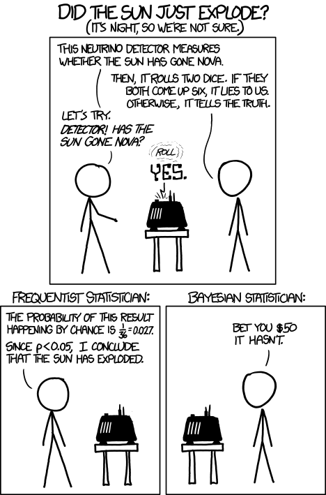
The null hypothesis
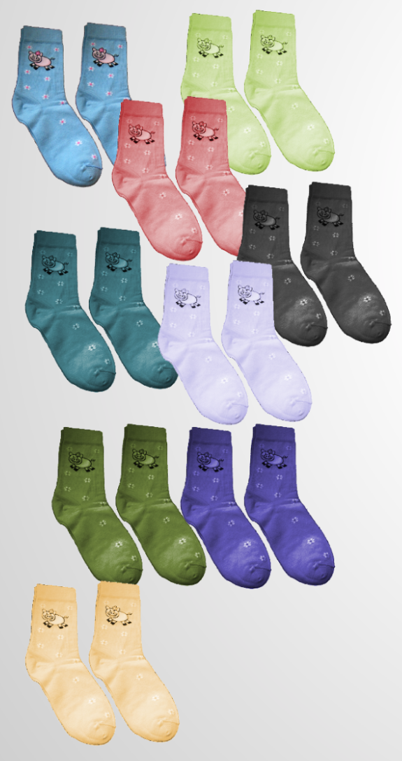
\[N_{pairs} = 9\]
The null hypothesis
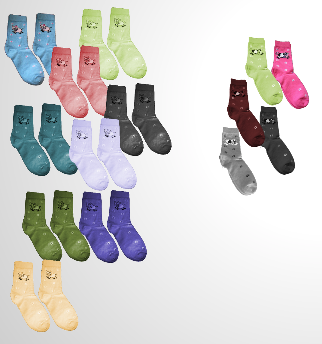
\[N_{pairs} = 9; \quad N_{singles} = 5\]
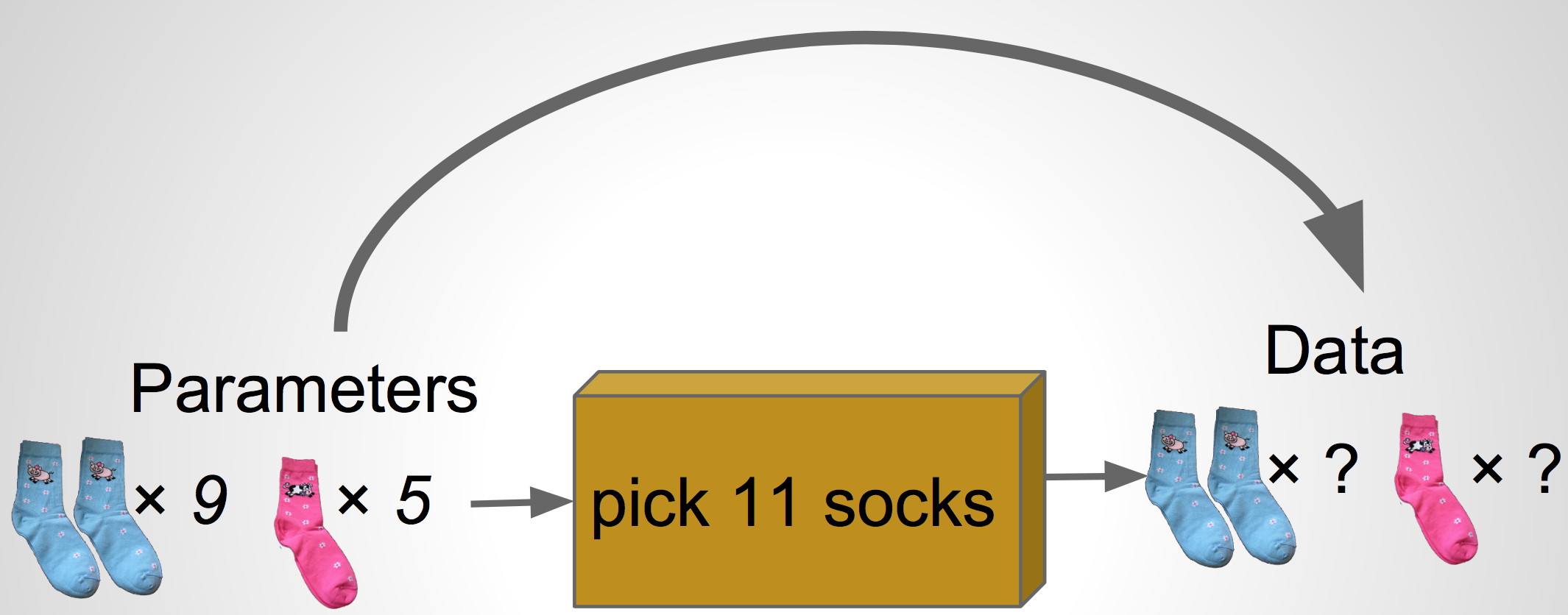
Our simulator
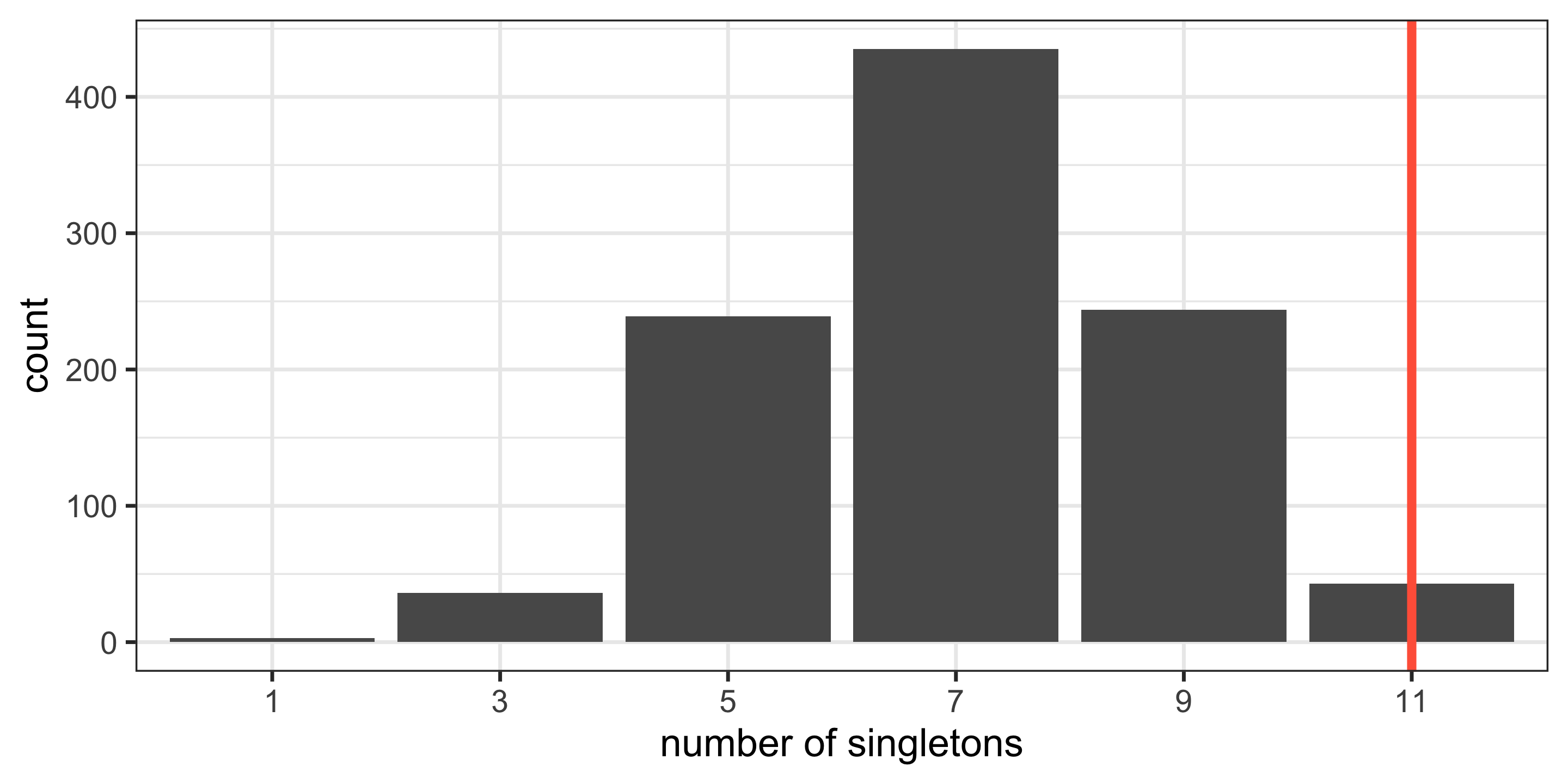
The null distribution
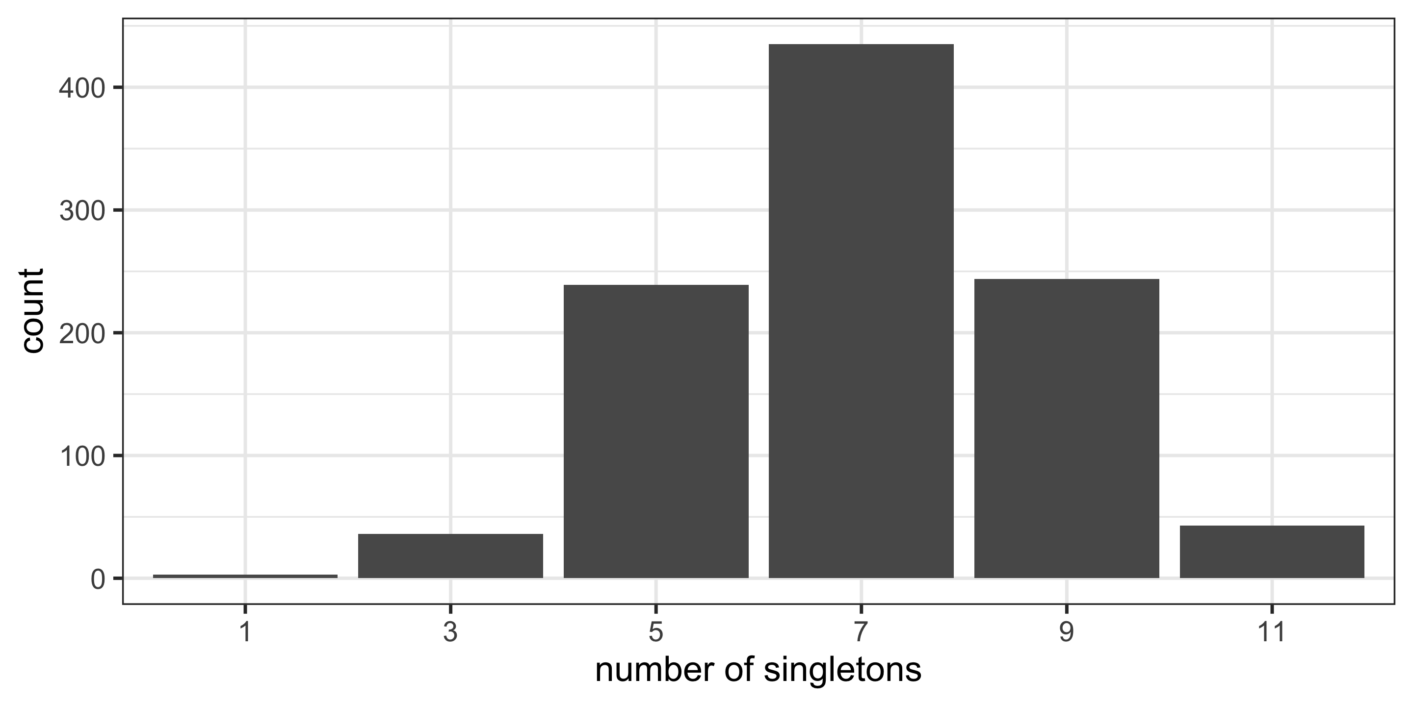
The null distribution
What we have
What we want
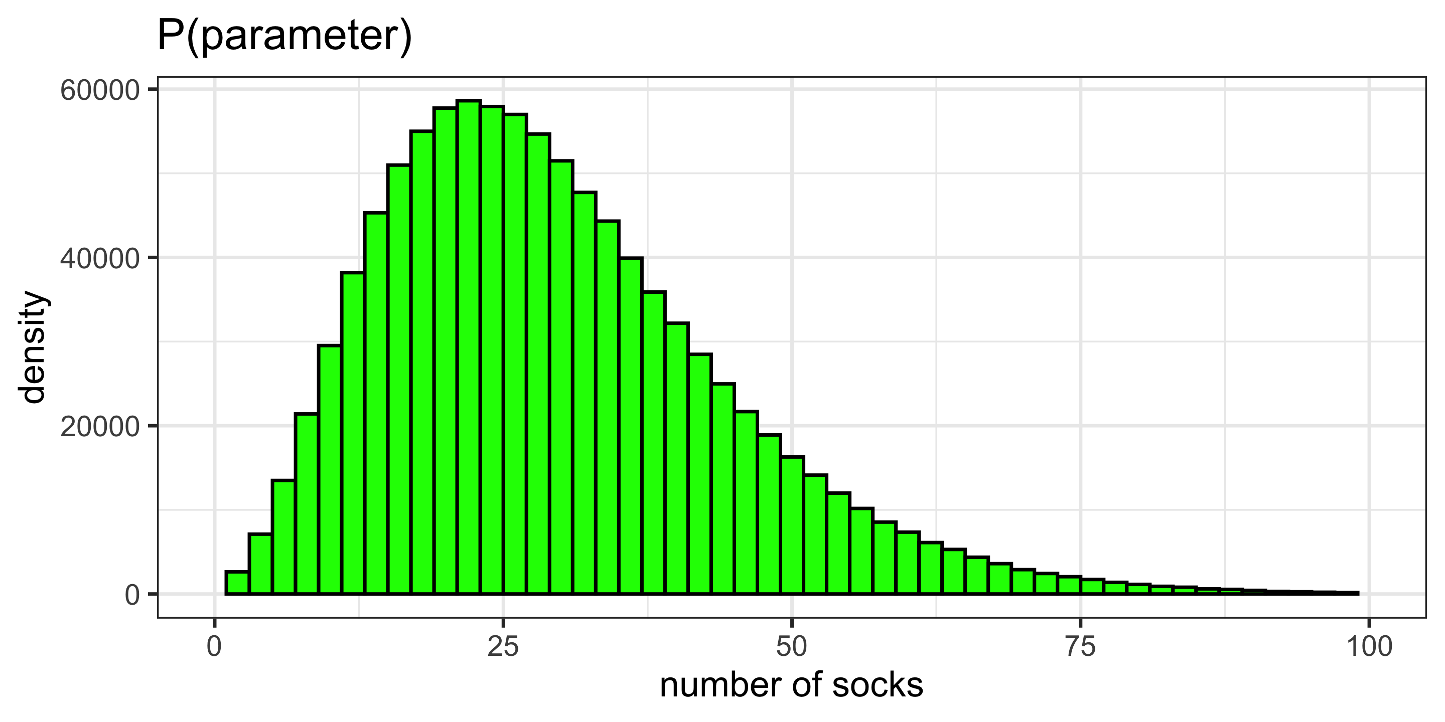
Prior distribution
A prior distribution is a probability distribution for a parameter that summarizes the information that you have before seeing the data. Prior on \(N\):
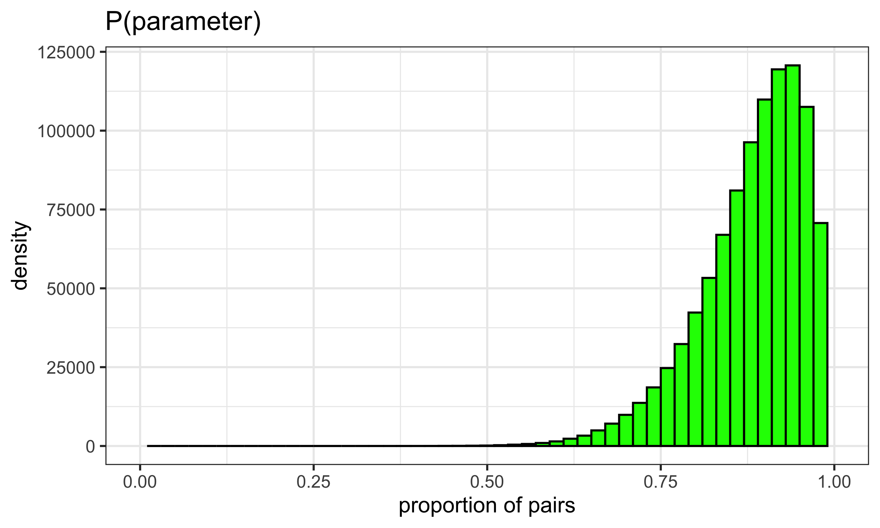
Prior on proportion pairs
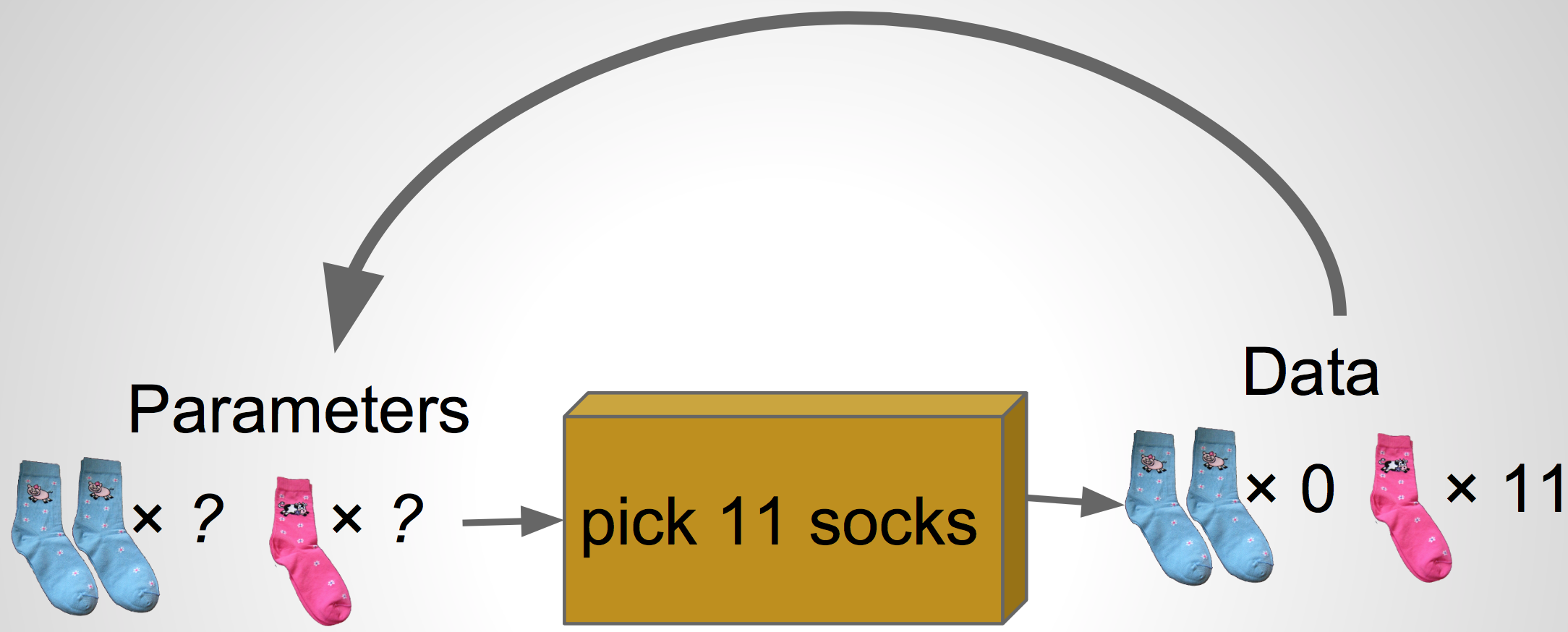
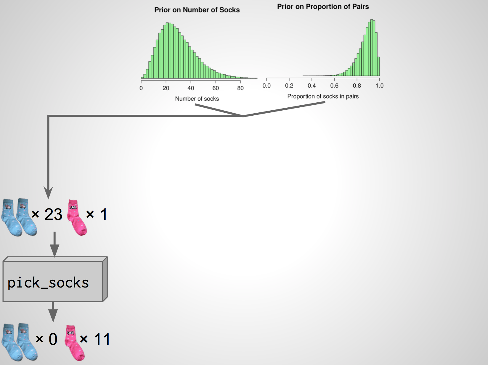
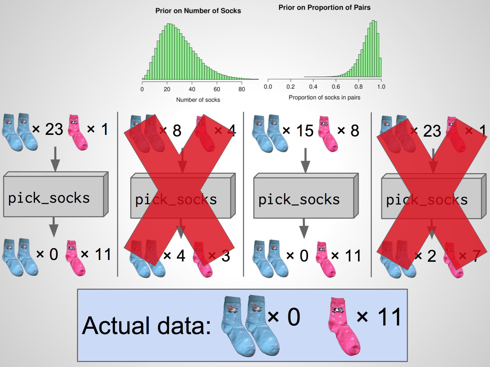
Our scheme
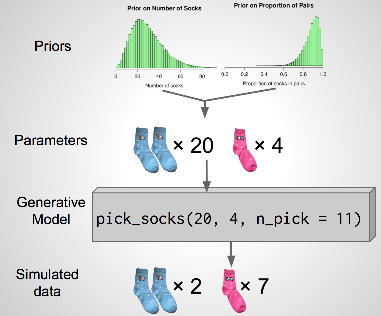
One simulation
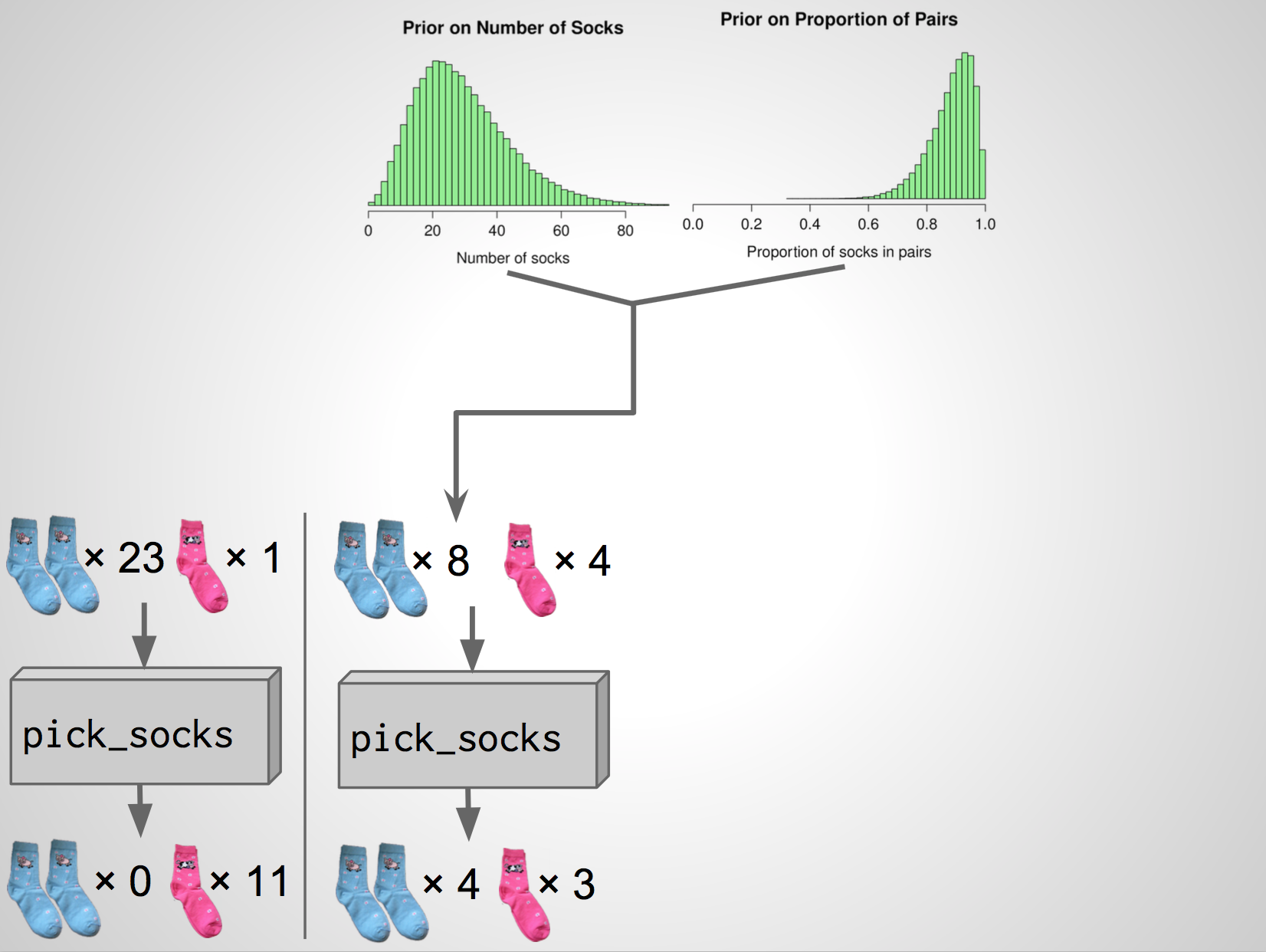
A second simulation
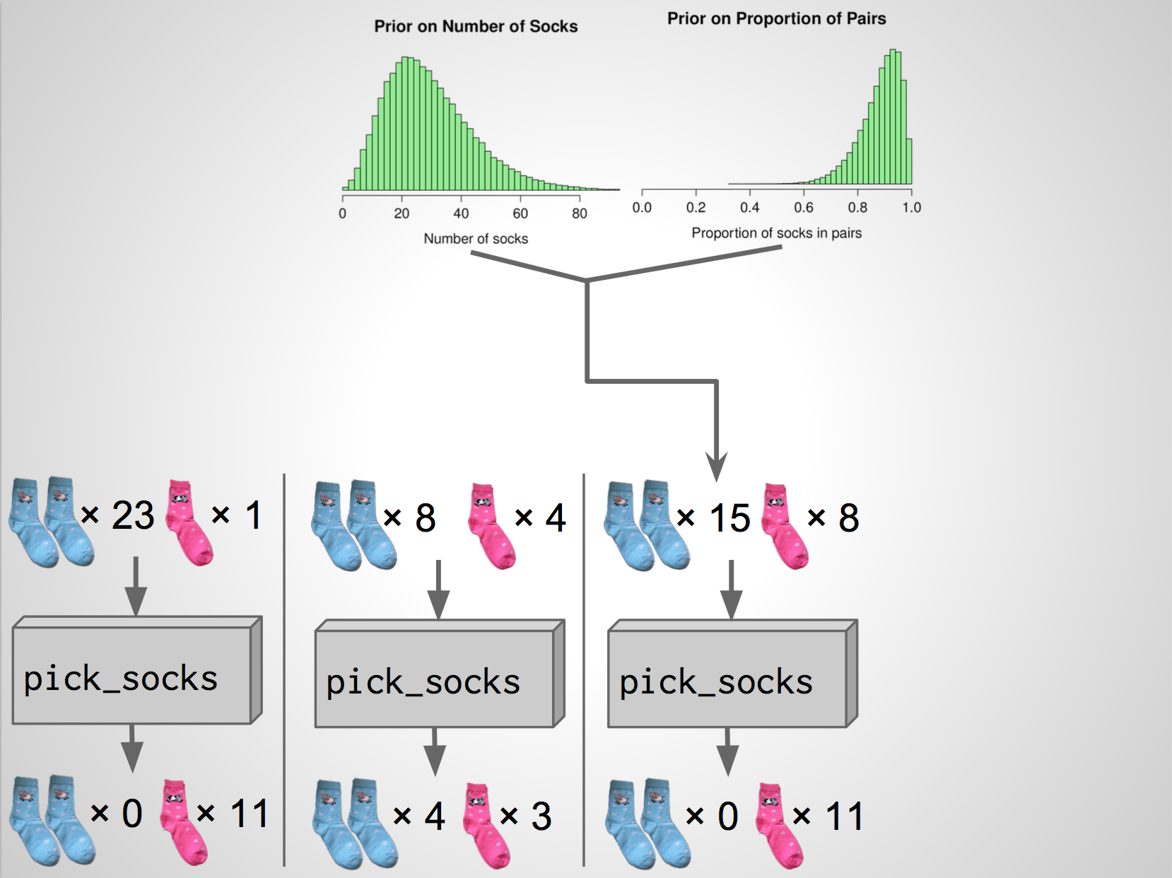
A third simulation
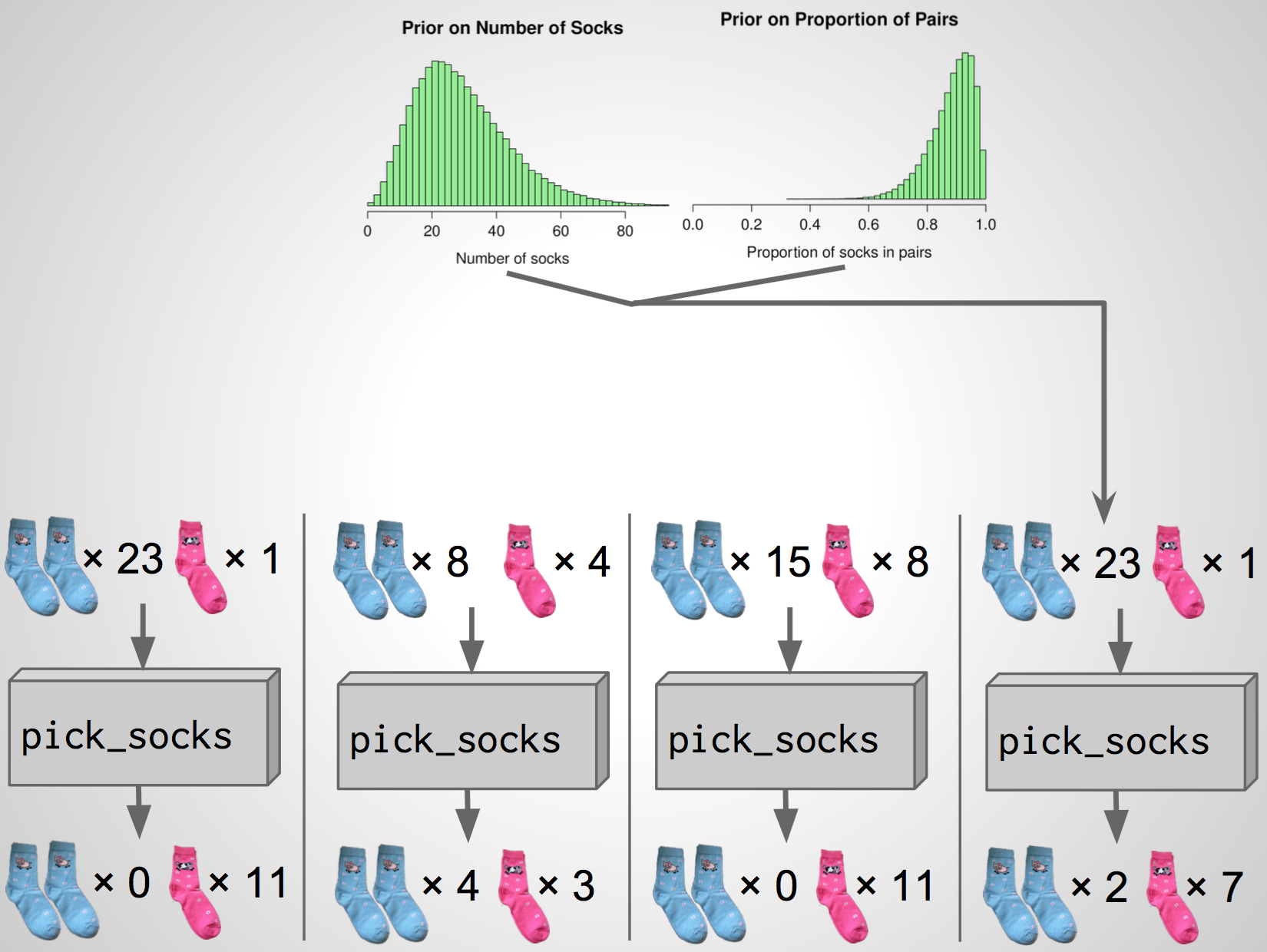
A fourth simulation
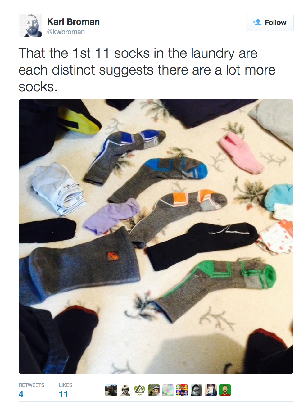
The actual data
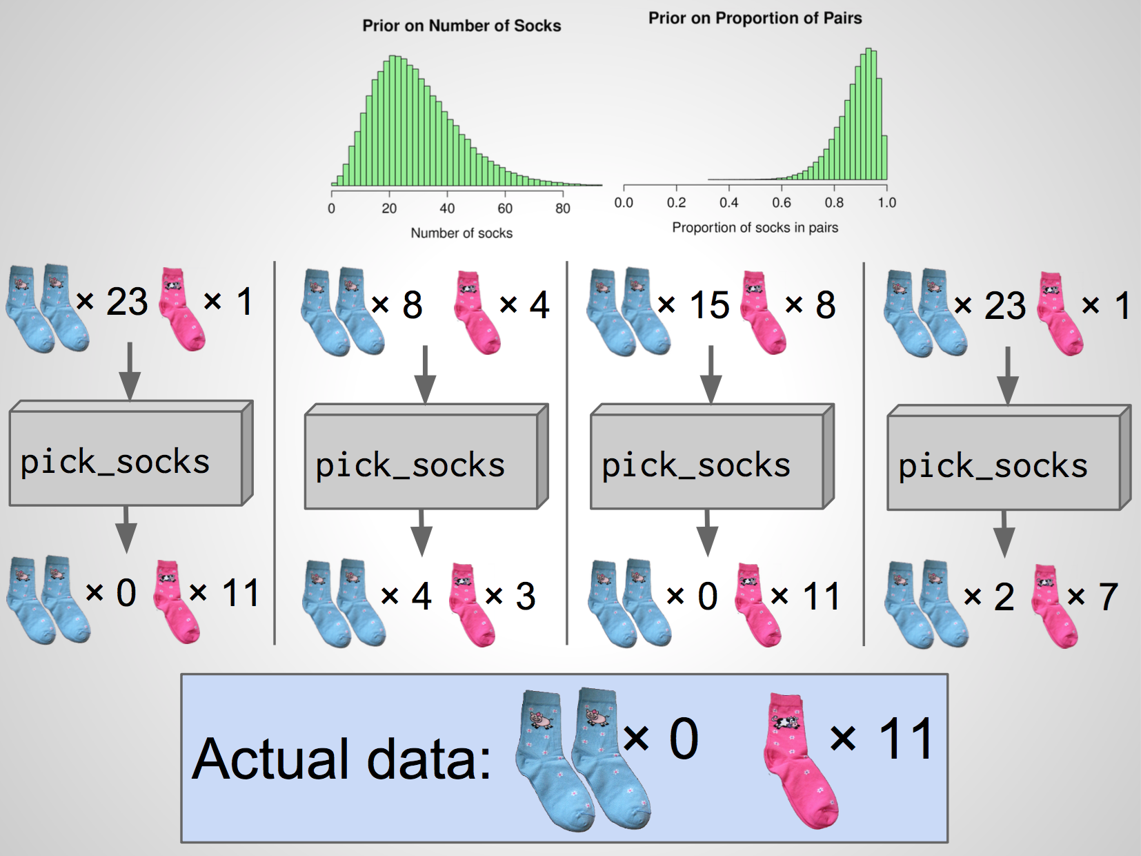
The actual data
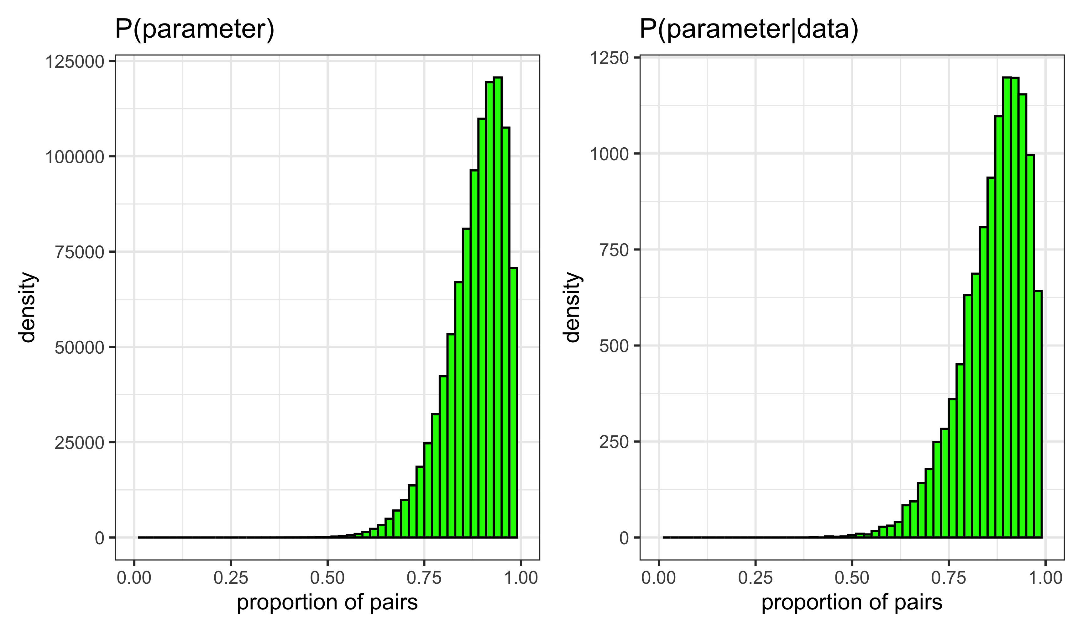
Proportion of pairs
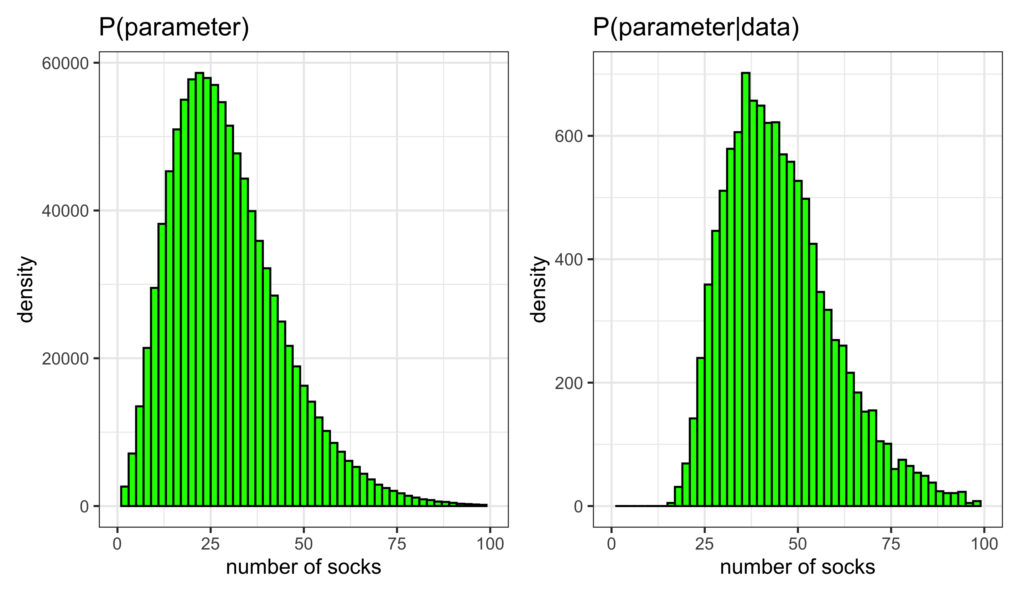
Number of socks
Karl Broman’s socks
The posterior distribution

- Distribution of a parameter after conditioning on the data
- Synthesis of prior knowledge and observations (data)
Question
What is your best guess for the number of socks that Karl has?
Our best guess
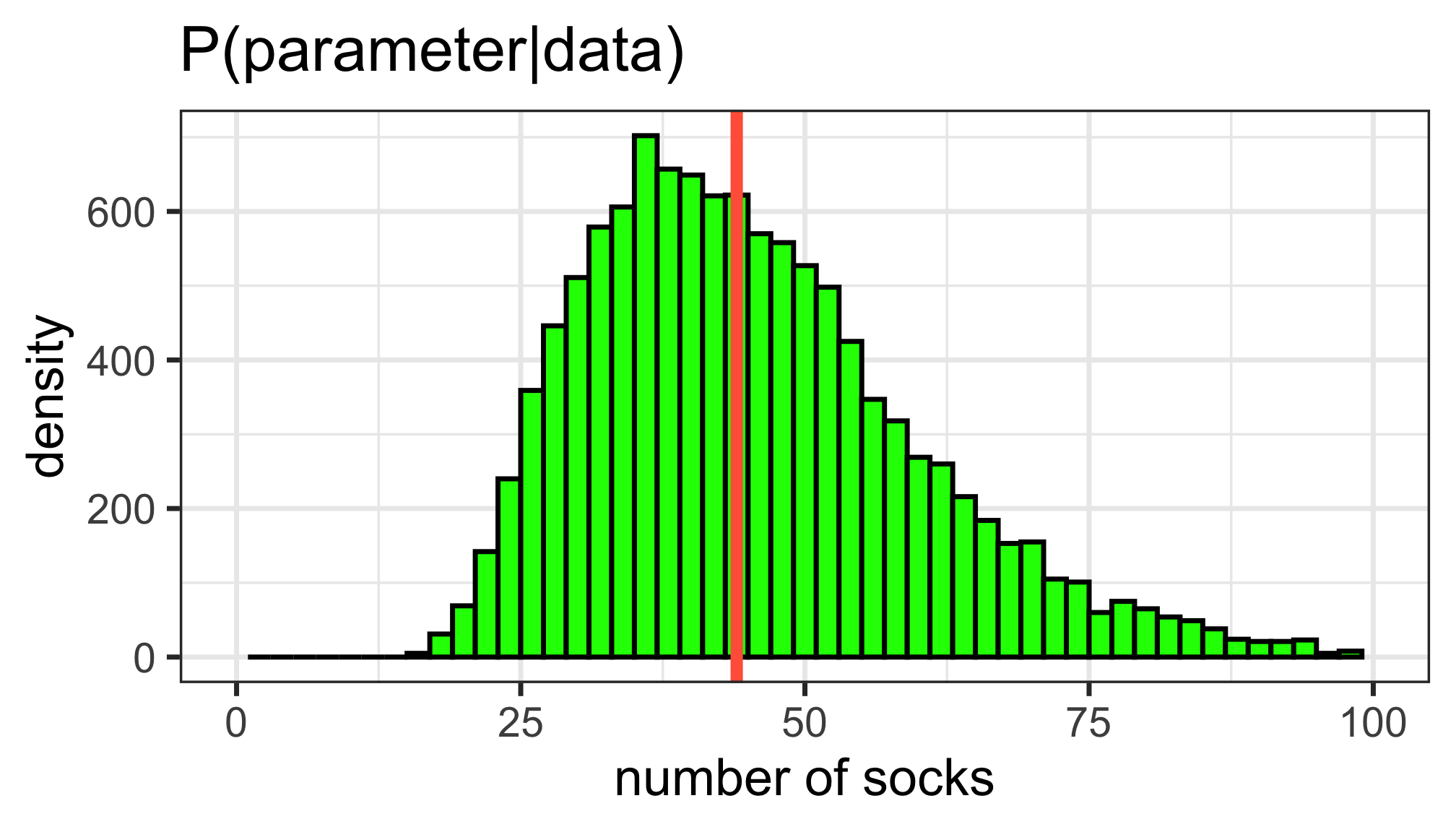
- The posterior median is 44 socks.
Karl Broman’s socks
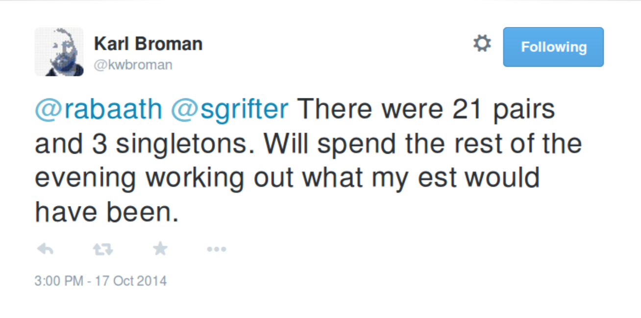
\[ 21 \times 2 + 3 = 45 \textrm{ socks} \]